16 November 2021

Inkscape has amazing svg path boolean logic functionality contained in the “livarot” source directory. My pylivarot project is an attempt to make this functionality within python.

For this project, I don’t want to distribute a source distribution, because pylivarot has many dependencies which can be challenging for a non-C++ developer to set up. I ran into a few issues creating binary distributions:

Cmake, setup.py and multiple versions of python

Martino Pilia has a great blog post about how to use cmake with setuptools, and my setup.py file is largely based on the example he worked with. However, I added a few extra hacks. The first is that the cmake FindPython cmake module doesn’t have enough granularity about python versions, so I wanted to get the library, include and executable from whatever python interpreter is currently running setup.py:

            extra_config_args = []
            extra_config_args.append(f"-DPYTHON_LIBRARIES={sysconfig.get_config_var('LIBDEST')}")
            extra_config_args.append(f"-DPYTHON_INCLUDE_DIRS={sysconfig.get_config_var('INCLUDEPY')}") # this might need to be the subdir
            extra_config_args.append(f"-DPYTHON_EXECUTABLE={sys.executable}")
            subprocess.check_call(['cmake', "-S", extdir]+extra_config_args, cwd=self.build_temp, env=env)

FindPython still needs to be called in order for pybind11_add_module and python3_add_library to be defined:

find_package(Python3 REQUIRED COMPONENTS Development)

C++17 symbols

  • pypi no longer accepts binary distributions that have the “linux” platform tag (it must be manylinux)
  • the manylinux debian image is docker 9, which only has GCC 6
  • lib2geom, one of my dependencies, uses std::optional, which is only available with C++17 forward
  • C++17 requires at least GCC 8, and will require the CXXABI_1.3.11 symbol
  • CXXABI_1.3.11 is not available for glibc 2.24, which is the latest version of glibc available through PEP 600

The solution here is to:

  1. install gcc-8 in the manylinux_2_24 docker image:
RUN apt install -y dirmngr && apt-key adv --recv-keys --keyserver keyserver.ubuntu.com 1E9377A2BA9EF27F && \
  echo "deb http://ppa.launchpad.net/ubuntu-toolchain-r/test/ubuntu xenial main" >> /etc/apt/sources.list && \
  apt-get update && apt-get install -y --no-install-recommends gcc-8 g++-8
  1. statically compile libg++:
set(CMAKE_CXX_FLAGS "-static-libstdc++")
  1. make sure that GCC 8 is being used within the pip virtual environment by putting in setup.py
            if os.path.exists('/usr/bin/gcc-8'):
                env['CC']='/usr/bin/gcc-8'
            if os.path.exists('/usr/bin/g++-8'):
                env['CXX'] = '/usr/bin/g++-8'
			subprocess.check_call(['cmake', "-S", extdir]+extra_config_args, cwd=self.build_temp, env=env)
  1. dump any extra shared objects into the whl directory before it is packaged:
        # copy all the built files into the lib dir. Not sure why this is needed; it feels like setuptools should 
        # copy the built files into the bdist by default
        lib_dir = os.path.join(self.build_lib, "pylivarot")
        for _file in glob(os.path.join(self.build_temp, f"*{sys.version_info.major}{sys.version_info.minor}*.so")):
            print("copying ", _file," to ", os.path.join(lib_dir, os.path.basename(_file)))
            shutil.move(_file, os.path.join(lib_dir, os.path.basename(_file)))
04 January 2021

Cricut Design Space, the software used to send designs to Cricut cutting plotters, does not handle the transform element on svg very well, which is frustrating because Inkscape loves to render paths with that attribute, rather than applying the transform directly to the path or object.

For example, here’s a design I made in inkscape. It has one path object representing the cuts I want to make in a piece of yellow cardstock on the bottom layer, and one group of paths to be traced out with a marker on the top layer:

a screenshot from inkscape

However, this fails to render correctly in Cricut Design Space:

failed render

The telltale sign about why this is rendered like this is to look at whether a transformation matrix is being applied to this element:

    <g
       id="g6018"
       transform="matrix(0.3071252,0.01878458,-0.01878458,0.3071252,92.391111,151.00958)"
       style="stroke-width:0.831982;stroke-miterlimit:4;stroke-dasharray:none">

There are also transforms applied to layers:

  <g
     inkscape:label="Layer 1"
     inkscape:groupmode="layer"
     id="layer1"
     transform="translate(-24.058,-19.5223)"
     style="display:inline">

Some transforms Cricut Design Space can handle okay, but some it cannot. A way I fixed the transforms on this project was:

  1. put all elements on the same layer
  2. ungroup the line patterns, then group them again

Now it renders as expected:

after group removal

Cricut also can’t handle the rotate transform. For example, I created a tiling that uses the rotate transform to put the trapezoids in the right place. But in Cricut, the trapezoids ignore this rotation, and all stack on top of each other:

rotation parsed badly

Unfortunately, there’s no ungrouping as a way to get out of this. Fortunately there’s a really nice extension called Apply Transforms that will take the the transform and apply it to the path itself. Now the tiling renders correctly:

rotation parsed correctly

08 June 2020

My great-grandmother Eudora was a calculus instructor at Ohio State and a fan of Martin Gardner’s Mathematical Games column in Scientific American. One of the concepts that Gardner introduced to a larger audience were Polyominos, extrapolation of dominos with larger numbers of squares. The shapes in Tetris are pentominos; they are shapes made up of 5 squares.

Eudora introduced Gardner’s column to my mother, Donna, who was also became a fan of recreational mathematics. In November, 1987, she saw this article in Science News:

Pieces of a Polyomino Puzzle

Polyominoes, which are the basis for thousands of mathematical puzzles, are shapes that cover connected squares on a checkerboard. One of the most intriguing of such puzzles involves proving that polyominoes of a certain shape can be laid down to form a complete rectangle. Recently. software engineer Karl A. Dahtke of AT&T Bell Laboratoties in Naperville, Ill., combining perseverance with clever computer programming, managed to solve two particularly perplexing versions of this problem — ones that for nearly 20 years had defeated the best efforts of scores of amateur and professional mathematicians. "I was amazed," says mathematician Solomon W. Golomb of the University of Southern California in Los Angeles, who in 1954 introduced the term "polyomino". Golomb has been exploring polyomino properties and proposing polyomino puzzles ever since. "A lot of very bright people have worked on [the problem]" he says. "This is a noteworthy accomplishment."

Dahlke, who is blind, first learned of the puzzles earlier this year in an audio edition of Science News. Dahlke spent several months working on the puzzles in his spare time. First, he tried proving that the problem has no solution. Because that approach didn't seem to lead anywhere, he started looking for an answer but kept running into dead ends. "I took so many different avenues," he says.

Finally, Dahlke decided to program his personal computer to search for an answer systematically. Dahlke's computer is equipped with a speech synthesizer that converts the computer's output into sound. It took the addition of several programming tricks designed to circumvent time-consuming situations, in which the computer was trapped in endlessly repeating patterns, before Dahlke found his two minimum-area rectangles (see illustrations).

"It turns out that the size of the solutions is clearly a little bit beyond what people could easily do by hand," says Golomb, "but fortunately, it's within the range of what you can find on a personal computer"

"I'm no Einstein," says Dahlke. "Maybe anyone with a micro, some perseverance and a little bit of geometric knowledge could have done it. But I did it, and it's a pretty thing."

Dahlke is ready to try more polyomino puzzles, He also dreams of the day when he'll get achance to go back to college to study mathematics at the graduate level.

image of the article in science news above

My mom made quilts of these two tilings between 1987 and 1989, which was impressive because I was born between the two quilts.

photo of my mom's two quilts

The quilts hung in the dining room of my childhood home. I spent many hours staring at them instead of practicing piano (sorry mom). When my parents downsized after retirement, they gave me the quilts, and they now hang in my bedroom. My baby loves looking at the quilts because they are bold colours with sharp edges. As a project while my baby sleeps in my lap, I have been translating/recreating Dahlke’s original C code into Python so that I can generate vectors of the tiling for use with a die cutter, embroiderer, etc.,

Dahlke has hosted his pentomino packing code on his website, but not, as far as I know, the code that originally generated the heptomino/hexonimo tilings above. I used the packing algorithm in Dahlke’s pentomino code but with the 8 orientations of the piece instead of all permutations of the pentominos and their orientations. The packing algorithm is:

  1. create a grid with a margin of size 2 around the edges. Fill the margins with a negative character.
  2. find the topmost leftmost unoccupied location in the grid, and see if any pieces, defined my their topmost leftmost square, can be placed in the board. The margins prevent pieces from being placed partially off the edge of the board.
  3. if no piece can fit, remove the last placed piece, and repeat step 2 with the next unused piece
  4. if there are no more empty locations in the grid, the board must be filled, therefore we have a solution

Using a single thread of my core i7 7700k, this algorithm takes 3.5 hours to find the hexomino solution, and 7 hours to find the heptomino solution. Given that this code took 3 days in the late eighties, and consumer grade computing hardware has grown exponentially in the meantime, this time is a bit disappointing. Granted, I have not studied the problem for nearly as long as Dahlke, so there are probably several things I could do to constrain the search space, which I suspect is what Dahlke did.

Here’s somethings I tried to cut down on the execution time:

  • parallelization: This problem does not have an obvious way to divide the search space evenly, so does not parallelize easily. I could use an evaluation queue for potential solutions, but the time cost of passing information between processes eclipses the time to evaluate each placement.

  • CSPs: I tried formulating the problem as a constraint satisfaction problem, to take advantage of numerical optimization techniques that have been developed since the 80s, but this ran for days without finding a solution. I suspect I haven’t set up all the necessary constraints.

  • removing holes: there are some placements that create holes that obviously can’t be filled by another shape. For example, if you place this heptomino sunny-side-up will create a hole in the next column that can’t be filled in by any piece:

placement of a piece that creates a hole

Thus, if the grid location two up and one to the right of the current location to be filled is occupied, this sunny-side-up piece can’t be placed. This cuts down the search space. I identified at least one grid location to check per piece orientation for the heptominos. This cut down the time to find the first solution to 1 hour. However, identifying and coding these rules is time consuming. It feels like there should be a way for the computer to automatically detect hole-creating placements, but I haven’t found how.

My code is available on github. Dahlke requested that his pentomino packing code be used only for personal use, thus these scripts are distributed with the Creative Commons Attribution-NonCommercial 3.0 Unported (CC BY-NC 3.0) license.

hexomino tiling

21 April 2020

freesewing.org maintains a node/react based editor for drafting parametric sewing patterns with JavaScript and JSON. Here are three ways to get it working on Windows:

Run on WSL

  • Download Ubuntu for Windows,
  • install node and npm via nvm, because the debian package for node is a bit old.
  • add
     watch: {
      chokidar: {
     usePolling: true
      }
    }
    

    to rollup.config.js in order for file changes to be picked up

  • If you want to use an editor in Windows to modify your patterns, open the files in Ubuntu file system mount point, which is going to be in *C:\Users<your windows username>\AppData\Local\Packages\CanonicalGroupLimited.UbuntuonWindows_\LocalState\rootfs\home\\\* . Once you edit these files in Windows, you will need to add linux file permissions back to your file, i.e. by running `sudo chmod 777 /src/index.js`

Things that didn’t work for me

running natively

For some reason npm link does not correctly create symlinks on Windows. Between running npm start in the main pattern folder, and npm start on the example folder, manually create the symlink, i.e.:

npm start
mklink /D "C:\<path to your pattern>\example\node_modules\pattern" "C:\<path to your pattern>"
cd example
npm start

This leads to some weird errors with stale code.

Running in a Docker container

Running in a docker container prompts some interesting problems:

  • nvm requires several environment variables to be set in order to work, but due to the idempotency of commands in dockerfiles, we can’t preserve these environment variables between steps. This means we need to explicitly state the node version and installation directory:
    ENV NVM_DIR /usr/local/nvm
    ENV NODE_VERSION 12.16.2
    RUN mkdir $NVM_DIR
    RUN curl -o- https://raw.githubusercontent.com/creationix/nvm/v0.34.0/install.sh | bash
    RUN [ -s "$NVM_DIR/nvm.sh" ] && \
      \. "$NVM_DIR/nvm.sh" && \
      [ -s "$NVM_DIR/bash_completion" ] && \
      \. "$NVM_DIR/bash_completion" && \
      nvm install $NODE_VERSION && \
      nvm alias default $NODE_VERSION && \
      nvm use default
    ENV PATH=$PATH:$NVM_DIR/versions/node/v$NODE_VERSION/bin
    
  • should we install npm dependencies at every run of the image? This will significantly increase the runtime. To save time, in my dockerfile I install all the dependencies globally:
    RUN npm install -g create-freesewing-pattern
    RUN curl -o example/package.json https://raw.githubusercontent.com/freesewing/freesewing/master/packages/create-freesewing-pattern/template/default/example/package.json
    RUN cd example && cat package.json | jq '.devDependencies' | sed 's/: /@/' | sed 's/"//g' | sed 's/,//' |sed 's/{//'| sed 's/}//' |xargs npm install -g --loglevel=error
    
  • do we run the server for both the editor front-end and pattern generator in the same line? I’ve never attempted to attach to a docker process in two different windows, so I run both in the same line, which puts all output in the same window.

For all of these complications, I ended up using the WSL instead.

01 August 2019

If you want a python script to automatically shut itself down if it uses a certain amount of memory, the internet will tell you to use the setrlimit function in the resource library:

import resource
MAX_MEMORY = 10_737_418_240 # the maximum memory in bytes that this process can use
rsrc = resource.RLIMIT_DATA
soft, hard = resource.getrlimit(rsrc)
resource.setrlimit(rsrc, (MAX_MEMORY, MAX_MEMORY))

This works fine on Solaris, but not on Linux or AIX systems. AIX does not have an RLIMIT_DATA metric. Instead, the RLIMIT_AS is a kind of similar measure of all heap allocated memory:

rsrc = resource.RLIMIT_AS if sys.platform.find('aix') == 0 else resource.RLIMIT_DATA

Linux is able to bypass the ulimits when allocating heap memory using mmap. If your script has a running event loop, for example, if it reads in a file line by line, then you can periodically check the memory:

usage = resource.getrusage(resource.RUSAGE_SELF).ru_maxrss
if usage > MAX_MEMORY/1024:
	raise ValueError(f'{sys.argv[0]} has exceeded the memory limit: {usage} > {MAX_MEMORY/1024}')

This is not ideal because it only alarms on the resident size, but there’s no fast way to check the virtual memory size: reading the maxrss takes microseconds, and opening and reading /proc/pid files takes tens of milliseconds. However, in most python programs, the difference between virtual and resident memory size is not that great.

For Windows, unless you compile a library that can load in and access the system DLs, there’s no fast way to check the memory. A slow way to check the memory is using the psutils library.

31 July 2019

How much memory does a python list require? This is easy to answer. Python has a function called getsizeof that will tell you directly:

>>> from sys import getsizeof
>>> getsizeof([1,2,3])
88

Okay, great, thanks Python! But why does this list take up 88 bytes? Also, if you run:

from sys import getsizeof
test_str = []
test_int = []
for i in range(100):
    test_int.append(i)
    test_str.append(str(i))
    print(i, getsizeof(test_int), getsizeof(test_str))

and plot the results, you’ll get:

a matplotlib graph of the size of a list of integers vs a list of strings

Why does a list of integers have the same reported size as a list of strings, when ‘1’ is larger than 1?

>>> getsizeof('1')
50
>>> getsizeof(1)
28

Why does the size increase in steps at a time, instead of strictly linear?

In the cpython listobject.c list_resize code, you can see that the memory for a list is allocated using the integer variable new_allocated :

    num_allocated_bytes = new_allocated * sizeof(PyObject *);
    items = (PyObject **)PyMem_Realloc(self->ob_item, num_allocated_bytes);

new_allocated is calculated using this formula:

    new_allocated = (size_t)newsize + (newsize >> 3) + (newsize < 9 ? 3 : 6);

newsize here is the requested resize of the list. When using append, this is going to be len(list)+1. new_allocated is always going to be larger than new_size. If you append to a list, and new_size is less than or equal to the already allocated size, the function returns early and memory is not reallocated. This is a time-saving feature; if you’re appending to a list, there’s a good chance you’re going to append to it again soon, so it doesn’t make sense to do the computationally expensive step of reallocating memory every time. This is why there’s a discrete rather than continuous trend between list size and allocated memory.

Let’s go over this step by step:

  • [].append(0) (1 + 1 » 3 + (1 < 9 ? 3 : 6) => (1 + 0 + 3) => 4
  • [0].append(1) 2<=4, do nothing => 4
  • [0, 1].append(2) 3<=4, do nothing => 4
  • [0, 1, 2].append(3) 4<=4, do nothing => 4
  • [0, 1, 2, 3].append(4) (5 + 5 » 3 + (5 < 9 ? 3 : 6) => (5 + 0 + 3) => 8

and so on.

We can also see that list_resize is allocating the size of a PyObject pointer, rather than the size of the object that you are appending to the list. Each item in a list exists elsewhere in memory, and the list just contains pointers to those items. If you want the true size of a list in python, you need to do recursively descend through each item in the list.

Finally, if you look at the cpython source code for getsizeof, you will see:

    if (PyObject_IS_GC(o))
        return ((size_t)size) + sizeof(PyGC_Head);

getsizeof adds on the memory cost of garbage collection. So, finally, the breakdown of that 88 bytes for the size of [1,2,3] on 64 bit systems is:

  • 40 bytes for the size of the list PyObject
  • 4 allocated size * 6 byte size of a PyObject pointer = 24
  • 24 bytes for garbage collection

On 32 bit systems, this is:

  • 20 bytes for the size of the list PyObject
  • 4 allocated size * 4 byte size of a PyObject pointer = 16
  • 12 bytes for garbage collection

Wow, garbage collection is expensive! Examining why is a separate post.

22 July 2018

My python automatic digitizer can now turn pngs, text, and a SVGs produced by a variety of software into computerized sewing machine embroidery patterns. However, I am hesitant to release and advertise this project because every other pattern ends up breaking a needle when loaded onto a sewing machine. Though needles are 25 cents each, it breaks the thread, and pieces of the need can end up lost under the base plate. My sewing machine manual suggests that this happens because there are three layers of threads.

I wrote some python code to measure the density of stitches. The heatmap looks like:

density of stitches

Some locations in the pattern have more than 7 points - and that location corresponds to the point where the needle breaks on the sewing machine. My strategy for reducing the density is discretize the pattern into a grid, and move the fourth stitch on every grid location to the next nearest grid location with fewer than three stitches. To do this, I create a generator:

# spiral around a point until you find the next available location
class NextAvailableGrid(object):
    def __init__(self, i, j):
        self.i = i # i is the x coordinate
        self.j = j # j is the y coordinate
        self.direction = "left"
        self.stepsize = 1
        self.current_step = 0

    def __iter__(self):
        return self

    def __next__(self):
        return self.next()

    def next(self):
        directions = ["left", "down", "right", "up"] # go counter-clockwise
        # do the transforms
        if self.direction == "left":
            self.i += 1
        if self.direction == "down":
            self.j += 1
        if self.direction == "right":
            self.i -= 1
        if self.direction == "up":
            self.j -= 1
        self.current_step += 1
        if self.current_step == self.stepsize:
            self.direction = directions[(directions.index(self.direction) + 1)
                                        % len(directions)]
            self.current_step = 0
            if self.direction in ["right", "left"]:
                self.stepsize += 1

        return self.i, self.j

This will spiral out from the grid location i, j forever:

grid spiral

Then, the code to move the stitches is:

def de_densify(pattern):
    density, boundx, boundy, x_bins, y_bins = initialize_grid(pattern)
    # convert the density list of lists to a dict
    density = {i: {j: block for j, block in enumerate(density[i])}
               for i in range(len(density))}
    for block_i, block in enumerate(pattern.blocks):
        for stitch_i, stitch in enumerate(block.stitches):
            i = int((stitch.x - boundx[1]) / minimum_stitch)
            j = int((stitch.y - boundy[1]) / minimum_stitch)
            # if there is room for that stitch, continue
            if density[j][i] <= MAX_STITCHES:
                density[j][i] += 1
                continue
            for next_i, next_j in NextAvailableGrid(i, j):
                if density[next_j][next_i] >= MAX_STITCHES:
                    continue
                print("moving stitch from {} {}".format(stitch.x, stitch.y))
                pattern.blocks[block_i].stitches[stitch_i].x = next_i * minimum_stitch + boundx[1]
                pattern.blocks[block_i].stitches[stitch_i].y = next_j * minimum_stitch + \
                                                               boundy[1]
                print("to {} {}".format(pattern.blocks[block_i].stitches[stitch_i].x, pattern.blocks[block_i].stitches[stitch_i].y))
                density[next_j][next_i] += 1
                break
    return pattern

The density map after moving the stitches is:

density of stitches after

And this gets stitched out without breaking a needle:

stitched out pattern

It’s still not where I want it - the jumps are too large and the threads cross over each other too frequently, but stitching without needle breaks is progress.

07 July 2018

I generate cairo tilings because I’m working on generating some custom printed fabric. Cairo tilings are an ideal pattern for clothing prints because they can be made from the same pentagon rotated to four different angles, yet still have a semi-regular repetition, meaning that you can clip the tiling at certain places, and copy that clip up and down to make an infinite pattern.

This post goes over my method of generating cairo tilings with minimal math using my fork of svgpathtools, and svgwrite. The full code to generate the tilings is available in my python-sewing repository.

Drawing the base pentagon

According to wikipedia, a cairo tiling can be made with a pentagon with the interior angles of 120, 90, 120, 120, and 90 radians. So I’ll start off with with an angle of 120 radians, and a length of 300 radians. I’m going to lay out my pentagon like this:

a single pentagon with annotated points

angle01 is the angle from horizontal to point 1 from point 0. I start with point 0 at 0,0:

def cexp(x):
    return pow(exp(1), x)
angle01 = 60.0
length1 = 300
# start with the top corner at 0, 0
points = [0, None, None, None, None]

Next, points 1 and 4 are at the projection up and down of angle01 from point 0:

points[1] = points[0] + length1 * cexp(1j * radians(angle01))
points[4] = points[0] + length1 * cexp(-1j * radians(angle01))

points 1 and 4 have interior angles of 90 degrees. To project up from these points, I subtract angle01 from 90:

angle12 = -(90 - angle01)
points[2] = points[1] + length1 * cexp(1j * radians(angle12))
points[3] = points[4] + length1 * cexp(-1j * radians(angle12))

I’ve drawn a single pentagon with minimal math - I only had to calculate the second projection angle, and the rest came from looking at the pentagon. I’m going to draw the four-groups of cairo tiling the same way.

Drawing the four-pentagon group

Next, I generate the 4-group:

4 group of pentagons

Like before with projecting from already-calculated points, I let svgpathtools do the work - use it to rotate the pentagons, snap them into place, then use the difference between where the points ended up for a list of transforms that I can use later.

def new_pentagon():
	return Path(*[Line(start=points[i - 1], end=points[i]) for i in range(len(points))])

transforms = [[0, 0]]
cairo_group = [new_pentagon()]
# point 1 of pentagon 1 needs to be attached to point 1 of pentagon 0
cairo_group.append(transform_path(rotate_transform(90), new_pentagon()))
diff = cairo_group[0][1].end - cairo_group[1][1].end
transforms.append([90, diff])
cairo_group[1] = cairo_group[1].translated(diff)
cairo_group.append(transform_path(rotate_transform(180), new_pentagon()))
# point 3 of pentagon 2 needs to be attached to point 2 of pentagon 0
diff = cairo_group[0][2].end - cairo_group[2][3].end
transforms.append([180, diff])
cairo_group[2] = cairo_group[2].translated(diff)
cairo_group.append(transform_path(rotate_transform(-90), new_pentagon()))
# point 4 of pentagon 3 needs to be attached to point 1 of pentagon 0
diff = cairo_group[0][4].end - cairo_group[3][4].end
transforms.append([-90, diff])
cairo_group[3] = cairo_group[3].translated(diff)

Finally, I want to calculate the width of the 4-group so that I know where to repeat the 4-group in the next step:

column_offset = cairo_group[0][0].end - cairo_group[1][2].end

Drawing the full pattern

The final trick to generating the full tiling is that every other 4-group in each row needs to be moved down by half of the height of the 4-group:

dwg = Drawing("{}/tiling2.svg".format(output_folder), profile="tiny")

current_color = 0
rep_spacing = pent_width * 2 + bottom_length

for y in range(num_down):
    transform = "translate({}, {})".format(0, rep_spacing * y)
    dgroup = dwg.add(dwg.g(transform=transform))
    for x in range(num_across):
        # if x is odd, point 0 of pent 0 needs to be attached to point 2 of pent 1
        if x % 2 == 1:
            dx = int(x / 2) * rep_spacing + pent_width * 2 + column_offset.real
            transform = "translate({}, {})".format(dx, column_offset.imag)
        else:
            transform = "translate({}, {})".format(int(x / 2) * rep_spacing, 0)
        group = dgroup.add(dwg.g(transform=transform))
        for pent in cairo_group:
            group.add(
                dwg.path(**{'d': pent.d(), 'fill': _colors[current_color % len(_colors)],
                            'stroke-width': 4, 'stroke': rgb(0, 0, 0)}))
            current_color += 1
dwg.save(pretty=True)

This generates the pattern:

Full tiling

10 May 2018

The common way to make modifications to sewing patterns is to trace out the cut lines on tracing paper, then cut and tape the pieces of paper together to form a new shape to cut out of fabric. However, as a software developer, every problem is a programming one, so in this post I’m going to show my code for extracting the cut lines from sewing patterns as SVGs, so that you can manipulate them in Inkscape.

The pattern I’m going to use in this demo is the Cheyenne Tunic by Hey June which I recommend purchasing. I use the pdfrw library for reading in the pattern, and investigating a pdf using this library can really help your understanding of the format.

Extracting data from PDFs is quite challenging. If you’re unfamiliar with PDFs, I recommend the O’Reilly book Developing with PDF.

Getting the Right Size

Most sewing patterns store the cut lines for different sizes in original content groups (known as layers in most PDF readers). This allows you to turn off the sizes you don’t want before printing.

the original content groups in the cheyenne tunic pattern

I set up a command argument parser to define the filename of the PDF and get the size to extract.

parser = argparse.ArgumentParser(
    description='Generate new pattern pieces from existing patterns')
parser.add_argument('--filename', type=str, help='The filename of the pdf pattern.')
parser.add_argument('--size', type=str, help="The size of the pattern to analyze.")

The content groups are defined both in the PDF document’s root, and on each page. The group keys for the content groups are defined under /Resources -> /Properties.

    args = parser.parse_args()
    x = PdfReader(args.filename, decompress=True)
    name = '(' + args.size + ')'
    shapes = []
    paths = []
    for page_num, page in enumerate(x.pages):
        if '/Resources' not in page:
            continue
        if '/Properties' not in page['/Resources']:
            continue
        oc_keyname = [key for key in page['/Resources']['/Properties']
                      if page['/Resources']['/Properties'][key]['/Name'] == name]

If there no original content groups matching the size we want, skip to the next page:

        if len(oc_keyname) == 0:
            continue

Another thing to extract out of the /Resources are the graphics states. If you want a faithful color representation of the graphics when converting PDF to SVG, you need these values. However, since these rules are a bit tricky, and I only care about the shapes, I am not doing anything meaningful with this information at the moment:

        gstates = {}
        if '/ExtGState' in page['/Resources']:
            gstates = page['/Resources']['/ExtGState']

The paths themselves will be in the page’s content stream. You want to start reading at the group key name, and then end at the end of that block, which is typically indicated by the EMC keyword:

        lines = page.Contents.stream.split('\n')
        start_index = [i for i, l in enumerate(lines) if l.find(oc_keyname) >= 0][0]
        end_index = \
        [i for i, l in enumerate(lines) if l.find('EMC') >= 0 and i > start_index][0]
        shape = "\n".join(lines[start_index:end_index])

PostScript Graphics to SVG

PDF graphics use a format similar to SVG for expressing shapes and paths, but uses a PostScript state machine for updating stylistic elements (like fill and stroke color) and for appending to paths. The instructions are written in reverse Polish notation, where the q operation pushes values onto the state machine and Q pops off the stack. I wrote a PostScript interpreter that goes over the instructions line by line, and adds shapes to a svgwrite Drawing. It’s by no means complete, but it’s good enough for my purposes. Some operators, like n, define clipping paths so that the cut lines render within the page window, and I ignore these.

def parse_shape(shape, i, gstates):
    # see https://www.adobe.com/content/dam/acom/en/devnet/acrobat/pdfs/PDF32000_2008.pdf
    output_filename = "page%s.svg" % i
    dwg = Drawing(output_filename, profile='tiny')
    fill = "none"
    stroke = rgb(0, 0, 0)
    stroke_width = 4
    transform = (1, 0, 0, 1, 0, 0)
    shapes_stack = []
    d = ""
    paths = []
    for line in shape.split("\n"):
        line = line.strip()
        parts = line.split(" ")
        nums = []
        for part in parts:
            try:
                nums.append(float(part))
            except ValueError:
                pass
        operation = parts[-1]
        if operation == 'BDC':
            continue
        elif operation == 'q':
            # q - start stack
            continue
        elif operation == 're':
            # rectangle
            vals = {'insert': (nums[0], nums[1]), 'size': (nums[2], nums[3])}
            if fill:
                vals['fill'] = fill
            if stroke:
                vals['stroke'] = stroke
            shapes_stack.append(dwg.rect(**vals))
        elif operation == 'n':
            # - clipping path
            continue
        elif operation == 'RG':
            # set stroke color
            stroke = rgb(*nums[0:3])
        elif operation == 'J':
            # not sure how to implement cap styles
            continue
        elif operation == 'cm':
            # current transformation matrix
            transform = nums[0:6]
        elif operation == 'F' or operation == 'f':
            # fill
            fill = rgb(*nums[0:3])
        elif operation == 'm':
            # move to
            d += "M " + format_pointstr(parts[0:2])
        elif operation == 'c':
            # curve
            d += " C " + format_pointstr(parts[0:6])
        elif operation == 'v':
            # append to bezier curve
            d += " S " + format_pointstr(parts[0:4])
        elif operation == 'y':
            d += " C " + format_pointstr(parts[0:4])+" "+format_pointstr(parts[2:4])
        elif operation == 'l':
            # line to
            d += " L " + format_pointstr(parts[0:2])
        elif operation == 'h':
            # make sure it's a closed path
            continue
        elif operation == 'S':
            # stroke to 4-unit width
            continue
        elif operation == 'Q':
            # end stack (draw)
            # apply transformation...
            for shape in shapes_stack:
                dwg.add(shape)
            if len(d) > 0:
                paths.append(d + " Z")
                d = " ".join([transform_str(p, transform) for p in d.split(" ")])
                vals = {'d': d}
                vals['stroke-width'] = stroke_width
                if fill:
                    vals['fill'] = fill
                if stroke:
                    vals['stroke'] = stroke

                dwg.add(dwg.path(**vals))
            d = ''
            shapes_stack = []
        elif operation == 'gs':
            key = parts[0]
            if key not in gstates:
                print("could not find state %s in dictionary")
            state = gstates[key]
            # color blending not yet implemented
            pass
        elif operation == 'w':
            stroke_width = nums[0]
        else:
            print("not sure what to do with %s %s" % (operation, line))
    dwg.save()
    return paths

PDF uses the same format as SVG for expressing transformations. Here’s my code for applying these transformations, which is copied from my fork of svgpathtools

def transform_point(point, matrix=(1, 0, 0, 1, 0, 0), format="float", relative=False):
    a, b, c, d, e, f = matrix
    if isinstance(point, list):
        x, y = point
    else:
        point_parts = point.split(',')
        if len(point_parts) >= 2:
            x, y = [float(x) for x in point_parts]
        else:
            # probably got a letter describing the point, i.e., m or z
            return point
    # if the transform is relative, don't apply the translation
    if relative:
        x, y = a * x + c * y, b * x + d * y
    else:
        x, y = a * x + c * y + e, b * x + d * y + f
    if format == "float":
        return x, y
    else:
        return "%s%s%s" % (x, point_separator, y)

Since the same cut lines are spread accross multiple pages, I want to eliminate duplicate cut lines, which I can do using set, since the shapes are all path strings:

paths = sorted(list(set(paths)))

Here’s all the unique cut lines for the XS shape:

all cut lines

Now that I have the cut lines in SVG format, I can programmatically manipulate them and then print them out again, but that’s a post for another day.

04 April 2018

Within five minutes of releasing the first version of my web interface to my python-embroidery package, embroidery-maker.com, it was broken by my first user uploading a PNG image instead of an SVG. Though SVGs are much easier to work with, as the list of stitches that gets sent to the sewing machine is much closer in data to a vector than a grid of pixels, I recognize that my user-base is more familiar with opening and editing PNGs than SVGs. Luckily adding support for PNGs was relatively painless thanks to the Potrace contour-tracing tool, and the python bindings.

First, I convert the individual pixels in the image into valid thread colors. At this point, it might also be useful to restrict the total number of colors in the image, which can be done using the Python Imaging Library’s convert method. My sewing machine seems willing to support an arbitrarily large number of different thread colors in patterns, but it can be a pain to have to take out and re-thread the machine many times.

def posturize(_image):
    pixels = defaultdict(list)
    for i, pixel in enumerate(_image.getdata()):
        x = i % _image.size[0]
        y = int(i/_image.size[0])
        if len(pixel) > 3:
            if pixel[3] == 255:
                pixels[nearest_color(pixel)].append((x,y, pixel))
        else:
            pixels[nearest_color(pixel)].append((x, y, pixel))
    return pixels

Next, I trace the image. Potrace can only handle two-color images, so I keep track of all of the thread colors, then go make a masked image with only the pixels of that thread color.

for color in pixels:
    data = zeros(_image.size, uint32)
    for pixel in pixels[color]:
        data[pixel[0], pixel[1]] = 1
    # Create a bitmap from the array
    bmp = potrace.Bitmap(data)
    # Trace the bitmap to a path
    path = bmp.trace()

Next, I want to convert this traced path into the svgpathtools curve objects, so that they can be used in the rest of the digitizer code as if it was parsed in from an SVG. I also need to keep track of the start locations of each segment, so that I can check whether the segment is a closed loop. If it is, I can add a fill and stroke color.

# Iterate over path curves
for curve in path:
    svg_paths = []
    start_point = curve.start_point
    true_start = curve.start_point
    for segment in curve:
        if true_start is None:
            true_start = segment.start_point
        if start_point is None:
            start_point = segment.start_point
        if isinstance(segment, BezierSegment):
            svg_paths.append(
                CubicBezier(start=start_point[1] + 1j * start_point[0],
                            control1=segment.c1[1] + segment.c1[0] * 1j,
                            control2=segment.c2[1] + segment.c2[0] * 1j,
                            end=segment.end_point[1] + 1j * segment.end_point[0]))
        elif isinstance(segment, CornerSegment):
            svg_paths.append(Line(start=start_point[1] + 1j * start_point[0],
                                  end=segment.c[1] + segment.c[0] * 1j))
            svg_paths.append(Line(start=segment.c[1] + segment.c[0] * 1j,
                                  end=segment.end_point[1] + 1j *
                                                             segment.end_point[
                                                                 0]))
        else:
            print("not sure what to do with: ", segment)
        start_point = segment.end_point
        # is the path closed?
        if true_start == start_point:
            output_paths.append(Path(*svg_paths))
            color = pixel[2]
            rgb = "#%02x%02x%02x" % (color[0], color[1], color[2])
            fill = rgb
            attributes.append({"fill": fill, "stroke": rgb})
            true_start = None
            start_point = None
            svg_paths = []

Then, I need to cut the shapes above out of the shapes below so that the SVG is only one layer deep.

Feeding these paths into my digitizer, it can turn PNG images like1:

the flag of Nova Scotia with an emoji cat face

into:

the flag of Nova Scotia with an emoji cat face, as a series of stitches

1: I’ve replaced the lion rampant on the flag of Nova Scotia with the emoji cat because it has too many curves to render nicely in stitches, and also because it amuses me

03 April 2018

SVGs will display the last added shape on top. This means you can very easily create the Canadian flag by layering a white rectangle on top of a red rectangle, but that correctly representing merged SVGs is difficult. It also means that, if you’re using SVGs to generate things in meatspace, like with a 3D printer, laser cutter or computerized sewing machine, you’re going to waste material and reduce the quality of the output. Before sending the SVG to the device, you’ll probably want to cut out the later shapes out of the lower shapes. Doing this is kind of tricky, and I’ll go over two methods that work, with trade-offs and one complicated method that I haven’t completed implementing. The code for this post is in my python-embroidery library.

Subtract the Paths

In SVGs, if you add one path string to another after the first string, SVG will render the second d string as a cut-out of the first d string. This means that you can go through the SVG paths and add the next two together:

for i in range(1, len(all_paths)):
    remove_path = all_paths[i].d()
    current_path = all_paths[i-1].d()
    all_paths[i-1] = parse_path(current_path+" "+remove_path)

This works well for shapes without the holes, so for example the shape:

svg rendering of a green star on a blue circle

will be cut into the shapes:

svg rendering of a green star cut out of a blue circle

However, for shapes that already have holes, like the shape:

svg rendering of a green star on a blue ring

will be cut into the shapes:

svg rendering of a green star cut out of a blue ring incorrectly

Cutting a path on an existing negative space turns it into a positive space. This makes sense if you have only an on or off setting for each fill area. So this method works well for simple shapes, but not for shapes that already have negative spaces. As soon as you try to stack multiple shapes, you’re going to be double-negating lots of shapes.

Use Computational Geometry

Computational Geometry is a tricky subject, luckily we can leverage that is used extensively in GIS code to avoid doing our own calculations. The Shapely python package has functions to perform all set operations on polygon points, including differencing. It doesn’t support curves, so you must first convert the SVG paths into polygons, do the difference, then convert the polygon into an SVG path:

from svgpathtools import Line, Path
from shapely.geometry import Polygon

def path_difference_shapely(path1, path2):
    # convert both paths to polygons
    def path_to_poly(inpath):
        points = []
        for path in inpath:
            if isinstance(path, Line):
                points.append([path.end.real, path.end.imag])
            else:
                num_segments = ceil(path.length() / minimum_stitch)
                for seg_i in range(int(num_segments + 1)):
                    points.append([path.point(seg_i / num_segments).real,
                                    path.point(seg_i / num_segments).imag])
        return Polygon(points)
    poly1 = path_to_poly(path1)
    poly2 = path_to_poly(path2)
    diff_poly = poly1.difference(poly2)
    points = diff_poly.exterior.coords
    new_path = []
    for i in range(len(points)-1):
        new_path.append(Line(start=points[i-1][0]+points[i-1][1]*1j,
                             end=points[i][0]+points[i][1]*1j))
    new_path.append(Line(start=points[-1][0]+points[-1][1]*1j,
                             end=points[0][0]+points[0][1]*1j))
    # make a new path from these points
    return Path(*new_path)

Here I’m sampling along any non-Line segments in the curve at intervals of minimum_stitch, which is the smallest stitch I’m going to tell my computerized sewing machine to make.

This cuts out our negative space the way we’d like:

svg rendering of a green star cut out of a blue ring correctly

Which is what we want. Unfortunately, doing this requires transforming our wonderful continuous Bezier curves into gross discrete polygons. This isn’t a problem if you know the lower resolution of the device that is going to render your SVG, like the minimum stitch of my sewing machine.

Use Inkscape

So what if you want to preserve your curves? Inkscape is able to do differences between shapes remarkably well, unfortunately their code for doing this is a thousand lines that is not linted, has no comments, and has methods and variables written in Franglish. Eventually, I’d like to understand what it is doing. Inkscape is a really wonderful tool and I understand that it is difficult to make a professional-level codebase on 0 income. If you want to just use Inkscape’s operations in your python code, you can use the inx-pathops package.

22 March 2018

If you want to use google’s cloud libraries so that you can take advantage bigquery or cloudstorage, you need to add them to the code you deploy with your app. Typically, I check out the repository to a lib directory, then put the lines:

import os
import sys
# path to lib directory
sys.path.insert(0, os.path.join(os.path.dirname(__file__), 'lib'))

in the file appengine_config.py.

This works when the code is deployed, but it doesn’t work locally, where the lib/google folder conflicts with the google-cloud-sdk/platform/google_appengine/google folder, resulting in the error:

ImportError: No module named google.cloud.bigquery

or

ImportError: No module named google.api_core

The solution I’ve found is to initialize the files lib/google/__init__.py and lib/google/cloud/__init__.py (so that the version of python running appengine can recognize these folders as packages) and then reload the google module in appengine_config.py:

import os
import sys
# path to lib directory
sys.path.insert(0, os.path.join(os.path.dirname(__file__), 'lib'))
# google needs to be reloaded so that it is taken from the 'lib' folder, and not the
# sandbox environment. Google needs to be loaded once to trigger python to look for the
# module
import google
reload(google)
# after reloading, trigger importing sub modules so that they are in the sys.modules
# dictionary in the correct location on future handlers
import google.api_core
import google.cloud
import google.cloud.bigquery

I’m not sure why this works, but it does.

01 February 2018

Most paper cutters, laser engravers, and 3D printers can’t handle fonts, and so ignore 〈text〉 tags in SVGs. Instead, text elements need to first be converted to paths by a program like Inkscape. This post describes how to automate text to path conversion in python using the freetype, svgpathtools, and svgwrite libraries.

I used the freetype rendering in matplotlib example as a guide.

First, load the svgpathtools paths, and define a tuple_to_imag function to convert between freetype’s tupple point representation to svgpathtools’ imaginary numbers:

from svgpathtools import wsvg, Line, QuadraticBezier, Path
def tuple_to_imag(t):
    return t[0] + t[1] * 1j

Load your font and initialize a character:

from freetype import Face
face = Face('./Vera.ttf')
face.set_char_size(48 * 64)
face.load_char('a')

We’ll be converting a string character by character. After converting this character to a path, you use the same method to convert the next character to a path, offset by the kerning:

face.get_kerning('a', 'b')

You’ll need to flip the y values of the points in order to render the characters right-side-up:

outline = face.glyph.outline
y = [t[1] for t in outline.points]
# flip the points
outline_points = [(p[0], max(y) - p[1]) for p in outline.points]

The face has three lists of interest: the points, the tags, and the contours. The points are the x/y coordinates of the start and end points of lines and control points. The tags indicate what type of point it is, where tag values of 0 are control points. Finally, the contours are the end point list index for each shape. Characters like i or ! have two shapes, most others have only one contour. So, for each contour, we want to pick out only the tags and points for that contour.

start, end = 0, 0
paths = []

for i in range(len(outline.contours)):
    end = outline.contours[i]
    points = outline_points[start:end + 1]
    points.append(points[0])
    tags = outline.tags[start:end + 1]
    tags.append(tags[0])

Next, we want to split the points up into path segments, using the tags. If the tags are 0, add the point to the current segment, else create a new segment, so that control points stay with their path segments:

    segments = [[points[0], ], ]
    for j in range(1, len(points)):
        segments[-1].append(points[j])
        if tags[j] and j < (len(points) - 1):
            segments.append([points[j], ])

Then convert the segments to lines. For lines with two control points (segment length 4), I could use the CubicBezier, but I find that breaking it into two Quadratic Beziers where the end point for the first and the start point of the second curve is the average of the control points, is more attractive:

    for segment in segments:
        if len(segment) == 2:
            paths.append(Line(start=tuple_to_imag(segment[0]),
                              end=tuple_to_imag(segment[1])))
        elif len(segment) == 3:
            paths.append(QuadraticBezier(start=tuple_to_imag(segment[0]),
                                         control=tuple_to_imag(segment[1]),
                                         end=tuple_to_imag(segment[2])))
        elif len(segment) == 4:
            C = ((segment[1][0] + segment[2][0]) / 2.0,
                 (segment[1][1] + segment[2][1]) / 2.0)

            paths.append(QuadraticBezier(start=tuple_to_imag(segment[0]),
                                         control=tuple_to_imag(segment[1]),
                                         end=tuple_to_imag(C)))
            paths.append(QuadraticBezier(start=tuple_to_imag(C),
                                         control=tuple_to_imag(segment[2]),
                                         end=tuple_to_imag(segment[3])))

Set the start location to the end location and continue. You can use the svgpathtools Path to merge the paths:

    start = end + 1

path = Path(*paths)
wsvg(path, filename="text.svg")

text.svg looks like:

You can see the full code in this gist.

21 January 2018

If you want to create or manipulate SVGs, there several great JavaScript libraries, such as d3 or Snap.js. However, right now I just want to stack a set of already-existing SVGs. I’ve created a gist with my code to stack SVGs, I’m going to go over it in this post.

This post assumes that the SVGs to stack are the strings of the file contents of the SVGs. You can acquire these strings by either reading in a user-supplied input file, or by making an HTTP request, but that is beyond the scope of this post.

Quick and Dirty

To extract the svg contents out of a string, you could do some string manipulations to strip everything up to the opening <svg> tag and after the closing </svg> tag. But since JavaScript was created with the goal of being able to manipulate XML files, this seems unnecessary. Instead, I use the DOMParser object to extract the SVG contents:

function getSVGContents(inputString){
    let domParser = new DOMParser();
    let svgDOM = domParser.parseFromString(inputString, 'text/xml')
        .getElementsByTagName('svg')[0];
    return svgDOM.innerHTML
}

Then, you can simply concatenate the strings:

document.getElementById("quickSVG").innerHTML =
         getSVGContents(circle)+getSVGContents(star);

SVGs have no z-index, like CSS. The elements that appear on the top are just the last elements to be added. So the above code would create the svg:

star over circle SVG

Whereas if you change the order of ‘circle’ and ‘star’ in the string concatenation:

document.getElementById("quickSVG").innerHTML =
         getSVGContents(star)+getSVGContents(circle);

The star will now be under the circle:

circle over star SVG

Less Quick, more OOPy

The above method is okay if you want to just layer the SVGs without manipulating them. But since we already have our strings parsed to DOM elements, we can combine the elements directly. We can initialize a SVG element, then use appendChild to move the child nodes from one element to another:

function addSVGs(inputStrings){
    // takes a list of strings of SVGs to merge together into one large element
    let svgMain = document.createElement("svg");
    for(let stringI=0;stringI<inputStrings.length;stringI++){
        let domParser = new DOMParser();
        let svgDOM = domParser.parseFromString(inputStrings[stringI], 'text/xml')
            .getElementsByTagName('svg')[0];
        while(svgDOM.childNodes.length>0){
            svgMain.appendChild(svgDOM.childNodes[0]);
        }
    }
    return svgMain

}
var svgMain = addSVGs([circle, star]);
document.getElementById("appendSVG").innerHTML = svgMain.innerHTML;

The things I found confusing about this method were:

  • first, unlike other XML parsers, DOMParser does not ignore whitespace. The tabs I put in to make my SVG strings more readable get read in as #text nodes. These strings will get rendered as whitespace, which don’t effect the final SVG.
  • appendChild removes the element from the input element’s parent, hence why it’s the first childNodes added to the mainSVG, and why I keep appending until there are no more childNodes in the svgDOM.
19 January 2018

If you’re building a Big Data application on AppEngine, you’ll probably need to grab more than a thousand entries out of a search index. It turns out this is not as straightforward as expected. I’ve built a sample project to demo how to do this.

In this demo we initialize our index to have 3000 entries of the numbers between 0 and 3000:

search_index = search.Index(name=INDEX_NAME, namespace=NAMESPACE)
for i in range(3000):
    fields = [search.NumberField(name='number_value', value=i),
              search.NumberField(name='last_modified', value=int(time()))]
    doc = search.Document(fields=fields)
    results = search_index.put(doc)

A first attempt at building a handler to query this index would be:

class Search(webapp2.RedirectHandler):
    def get(self):
        try:
            limit = int(self.request.get('limit'))
        except:
            limit = DOCS_PER_PAGE_LIMIT
        try:
            offset = int(self.request.get('offset'))
        except:
            offset = 0

        expr_list = [
            search.SortExpression(
                expression='number_value',
                default_value=int(0),
                direction=search.SortExpression.ASCENDING
            )
        ]
        sort_opts = search.SortOptions(expressions=expr_list)
        index = search.Index(name=INDEX_NAME, namespace=NAMESPACE)
        search_query = search.Query(
            query_string='',
            options=search.QueryOptions(
                limit=limit, sort_options=sort_opts, offset=offset, ids_only=False)
        )

This works well for values under 1000, but if you try to run the query /search?limit=3000, you’ll get the error:

Traceback (most recent call last):
  File "/home/catherine/installed/google-cloud-sdk/platform/google_appengine/lib/webapp2-2.5.2/webapp2.py", line 1535, in __call__
    rv = self.handle_exception(request, response, e)
  File "/home/catherine/installed/google-cloud-sdk/platform/google_appengine/lib/webapp2-2.5.2/webapp2.py", line 1529, in __call__
    rv = self.router.dispatch(request, response)
  File "/home/catherine/installed/google-cloud-sdk/platform/google_appengine/lib/webapp2-2.5.2/webapp2.py", line 1278, in default_dispatcher
    return route.handler_adapter(request, response)
  File "/home/catherine/installed/google-cloud-sdk/platform/google_appengine/lib/webapp2-2.5.2/webapp2.py", line 1102, in __call__
    return handler.dispatch()
  File "/home/catherine/installed/google-cloud-sdk/platform/google_appengine/lib/webapp2-2.5.2/webapp2.py", line 572, in dispatch
    return self.handle_exception(e, self.app.debug)
  File "/home/catherine/installed/google-cloud-sdk/platform/google_appengine/lib/webapp2-2.5.2/webapp2.py", line 570, in dispatch
    return method(*args, **kwargs)
  File "/home/catherine/python_projects/appengine-large-offset-example/main.py", line 55, in get
    limit=limit, sort_options=sort_opts, offset=offset, ids_only=False)
  File "/home/catherine/installed/google-cloud-sdk/platform/google_appengine/google/appengine/api/search/search.py", line 3073, in __init__
    self._limit = _CheckLimit(limit)
  File "/home/catherine/installed/google-cloud-sdk/platform/google_appengine/google/appengine/api/search/search.py", line 2858, in _CheckLimit
    upper_bound=MAXIMUM_DOCUMENTS_RETURNED_PER_SEARCH)
  File "/home/catherine/installed/google-cloud-sdk/platform/google_appengine/google/appengine/api/search/search.py", line 496, in _CheckInteger
    raise ValueError('%s, %d must be <= %d' % (name, value, upper_bound))
ValueError: limit, 3000 must be <= 1000

We can’t get all 3000 entries in one query, so we’ll have to spread the acquisition over three queries:

  • /search?limit=1000
  • /search?limit=1000&offset=1000
  • /search?limit=1000&offset=2000

The first two queries work, but if you set offset to 2000, you’ll get the error:

Traceback (most recent call last):
  File "/home/catherine/installed/google-cloud-sdk/platform/google_appengine/lib/webapp2-2.5.2/webapp2.py", line 1535, in __call__
    rv = self.handle_exception(request, response, e)
  File "/home/catherine/installed/google-cloud-sdk/platform/google_appengine/lib/webapp2-2.5.2/webapp2.py", line 1529, in __call__
    rv = self.router.dispatch(request, response)
  File "/home/catherine/installed/google-cloud-sdk/platform/google_appengine/lib/webapp2-2.5.2/webapp2.py", line 1278, in default_dispatcher
    return route.handler_adapter(request, response)
  File "/home/catherine/installed/google-cloud-sdk/platform/google_appengine/lib/webapp2-2.5.2/webapp2.py", line 1102, in __call__
    return handler.dispatch()
  File "/home/catherine/installed/google-cloud-sdk/platform/google_appengine/lib/webapp2-2.5.2/webapp2.py", line 572, in dispatch
    return self.handle_exception(e, self.app.debug)
  File "/home/catherine/installed/google-cloud-sdk/platform/google_appengine/lib/webapp2-2.5.2/webapp2.py", line 570, in dispatch
    return method(*args, **kwargs)
  File "/home/catherine/python_projects/appengine-large-offset-example/main.py", line 55, in get
    limit=limit, sort_options=sort_opts, offset=offset, ids_only=False)
  File "/home/catherine/installed/google-cloud-sdk/platform/google_appengine/google/appengine/api/search/search.py", line 3082, in __init__
    self._offset = _CheckOffset(offset)
  File "/home/catherine/installed/google-cloud-sdk/platform/google_appengine/google/appengine/api/search/search.py", line 2895, in _CheckOffset
    upper_bound=MAXIMUM_SEARCH_OFFSET)
  File "/home/catherine/installed/google-cloud-sdk/platform/google_appengine/google/appengine/api/search/search.py", line 496, in _CheckInteger
    raise ValueError('%s, %d must be <= %d' % (name, value, upper_bound))
ValueError: offset, 2000 must be <= 1000

Darn. Because of these limitations, we’re going to need a concept from Databases usually reserved for operations that span multiple computers: a cursor.

You can set as a parameter to the query options:

search_query = search.Query(
    query_string='',
    options=search.QueryOptions(
        limit=self.limit,
        sort_options=self.sort_opts,
        cursor=search.Cursor(per_result=False),
        ids_only=False,
    )
)

you can access the cursor for this search query after getting the results:

search_results = self.index.search(search_query)
cursor = search_results.cursor        

The strategy for pulling out the entries is this:

  1. create a search with no offset and a new cursor
  2. initialize current_offset to 0
  3. while current_offset is less than the desired offset, query the search index again with the cursor of the last query, and add the limit to the current_offset
  4. output the last search results

It would be nice if we could start our loop at the maximum offset in order to limit the number of repetitions of step 3, but if you do, you’ll get the error:

ValueError: cannot set cursor and offset together

Also, make sure that you set the per_result value of search.Cursor to False, or else the cursor will be None:

  File "/home/catherine/python_projects/appengine-large-offset-example/main.py", line 109, in query_with_cursors
    cursor_cache[current_offset] = search_results.cursor.web_safe_string
AttributeError: 'NoneType' object has no attribute 'web_safe_string'

Here’s the implementation:

current_offset = self.limit
search_query = search.Query(query_string='',
    options=search.QueryOptions(
        limit=self.limit,
        sort_options=self.sort_opts,
        cursor=search.Cursor(per_result=False),
        ids_only=False,
    )
)

search_results = self.index.search(search_query)
if self.offset >= search_results.number_found:
    return self.render_search_doc([])
while current_offset < self.offset:
    current_offset += self.limit
    search_query = search.Query(query_string='',
        options=search.QueryOptions(
            limit=self.limit,
            sort_options=self.sort_opts,
            cursor=search_results.cursor
        )
    )
    search_results = self.index.search(search_query)
self.render_search_doc(search_results)

Now, if we’re going to be querying an offset of up to 100000, it will take a while to do 1000 queries. So, it would be better if we could cache these cursors. We can stick the web_safe_string in memcache:

cursor_cache = {}
current_offset = self.limit
search_query = search.Query(query_string='',
    options=search.QueryOptions(
        limit=self.limit,
        sort_options=self.sort_opts,
        cursor=search.Cursor(per_result=False),
        ids_only=False,
    )
)

search_results = self.index.search(search_query)
cursor_cache[current_offset] = search_results.cursor.web_safe_string
if self.offset >= search_results.number_found:
    return self.render_search_doc([])
while current_offset < self.offset:
    current_offset += self.limit
    search_query = search.Query(query_string='',
        options=search.QueryOptions(
            limit=self.limit,
            sort_options=self.sort_opts,
            cursor=search_results.cursor
        )
    )
    search_results = self.index.search(search_query)
    cursor_cache[current_offset] = search_results.cursor.web_safe_string
memcache.set(cursor_cache_key, json.dumps(cursor_cache))
self.render_search_doc(search_results)

And then the next time, we can pull out the cursor for that offset:

cursor_cache_key = 'cursors'
cursor_cache = memcache.get(cursor_cache_key)
if cursor_cache:
    cursor_cache = json.loads(cursor_cache)
    offset_key = str(self.offset)
    if offset_key in cursor_cache:
        cursor_cache = cursor_cache[offset_key]
    else:
        logging.info("%s not in %s" %(offset_key, cursor_cache))
        cursor_cache = None

if cursor_cache:
    logging.info("found cursor cache string %s " % cursor_cache)

    # construct the sort options
    search_query = search.Query(
        query_string='',
        options=search.QueryOptions(
            limit=self.limit,
            sort_options=self.sort_opts,
            cursor=search.Cursor(per_result=False, web_safe_string=cursor_cache),
            ids_only=False,
        )
    )
    return self.render_search_doc(self.index.search(search_query))

A next step would be to find the nearest cursor offset, and start from there. But that would be another blog post.

14 December 2017

I have a dilemma: I don’t want to buy stuff for holidays, but I also don’t want to be the only house on my street without Christmas lights. So I made myself some Christmas lights from:

  • the leftover 5050 RGB LEDs from my last PC build
  • the 12 V DC power supply from my old wifi router
  • the leftover canvas from making a bike bag
  • a leftover dowel rod from making a bookcase

I made a model of an individual LED strip in Inkscape and experimented with a few designs. The one I ultimately chose was these snowflakes:

snowflakes made out of LEDs vector

I chose this design because it had relatively few angles, which meant I could free-hand layout the LEDs without needing to project the design onto the fabric:

photo of snowflakes made out of LEDs

I soldered the 12V and Blue Grounds on each snowflake, and then hot-glued some of the longer wires down to the fabric:

photo of snowflakes with lines soldered down

This is the end result:

photo of snowflake lights in window from the outside

26 November 2017

I recently purchased a Computerized Sewing Machine. Designs can be uploaded to internal storage via USB, which ubuntu automatically recognizes and mounts:

my ubuntu ultrabook and my brother sewing machine

This compatibility with linux out of the box is fantastic; unfortunately designs must be in Brother’s undocumented binary file format, and the sewing machine gives no feedback regarding parsing errors. This means that I’ve been creating binaries for embroidery patterns with a lot of trial and error. In order to script some of the process, I’d like to upload and test new designs without human intervention.

To find where ubuntu has mounted the sewing machine, I could either:

  1. write some udev rules
  2. get python to figure it out from linux commands

In this case, method 2 is a bit nicer since I’m already using Python to generate the binary files.

First, I use the output of df to generate a mapping of where ubuntu has mounted the external drives:

mount_points = {}
out = check_output(["df"]).split("\n")
for line in out:
    if line.find("/media") >= 0:
        mount_location = line.split("%")[-1]
        line = line.split(" ")
        mount_points[line[0]] = mount_location.strip()

Next, get the vendor ids for each device, and if it matches, call that my mount location:

mount_destination = None
for mount_point in mount_points:
    out = check_output(["udevadm", "info", "--name="+mount_point, "--attribute-walk"])
    if out.find('ATTRS{idVendor}=="04f9"')> 0:
        print("found brother device, assuming embroidery machine")
        mount_destination = mount_points[mount_point]
        break

So I can now use shutil.copyfile() to move the files over to mount_destination. This is kind of a hacky solution because it may also catch Brother printers, or fail to recognize embroidery machines from other manufacturers, but since I have neither of these situations, it’s good enough for now.

28 October 2017

My husband and I disagree about whether it’s more energy efficient to use the toaster oven or regular oven for baking. He believes the toaster oven consumes less energy, since the internal volume is much smaller. I believe the oven consumes less because it is better insulated.

I did some back-of-the-envelope calculations to see if there was an obvious conclusion. I estimate that the total power consumed is the work needed to heat up the volume of air inside the oven to the desired temperature, plus the work lost to heat transfer out of the door. It’s also possible that the heat is lost through the other sides, but I didn’t take that into account. From the ideal gas law, the work to heat up the air inside the oven is:

\[ W = D_mVR\triangle T \]

Where \(D_m\) is the molar density of air, \(V\) is the volume, \(R\) is the ideal gas constant, and \(\triangle T\) is the temperature change.

The heat lost through the oven door is:

\[ Q = kA\triangle Tt \]

Where \(k\) is the heat transfer coefficient, \(A\) is the area of the door, and \(t\) is the time that the oven is on.

Since both ovens have the same depth, the ratio of the ovens’ volume, 2.8, is the same for the door area. Some mechanical engineers estimate that the \(k\) of double-paned oven doors is ~3, whereas the toaster oven’s single pane of glass is 5.8. The ratio of these coefficients almost exactly cancels out the difference in volume. Because the heat is constantly being leaked out of the ovens, the work due to lost heat is nearly an order of magnitude larger than work required to heat up the oven, so this contribution can be mostly ignored. Since we don’t exactly know \(k\) for both ovens, we’re going to need to get experimental.

I bought an Aeotek Smart Energy Meter (currently on Amazon for 32 USD) and an Aeotek Z-stick (currently on Amazon for 45 USD)1. The Z-Stick is compatible with open-zwave which has a python interface.

My code to grab the power data on linux is:

import time
from openzwave.option import ZWaveOption
from libopenzwave import PyManager
import csv
from matplotlib import pyplot

device="/dev/ttyUSB0"
options = ZWaveOption(device, config_path="/etc/openzwave/", user_path=".", cmd_line="")
options.set_console_output(False)
options.lock()


class PowerMeter(PyManager):
    def __init__(self):
        super(PowerMeter, self).__init__()
        self.create()
        self.addWatcher(self.callback)
        time.sleep(1.0)
        self.addDriver(device)
        self.meter_values = []
        self.start_time = None
        self.units = None
        self.value_id = None

    def get_meter_values(self, num_seconds):
        self.start_time = time.time()
        while time.time() - self.start_time < num_seconds:
            time.sleep(0.10)
            if self.value_id:
                assert self.refreshValue(self.value_id)

    def callback(self, zwargs):
        # get measurement value from the first message tagged with the sensor we want
        if "valueId" in zwargs:
            if zwargs["valueId"]["commandClass"] == "COMMAND_CLASS_METER":
                if zwargs["valueId"]["label"] == "Power" and \
                                zwargs["valueId"]["instance"] == 1 \
                        and self.start_time is not None:
                    self.value_id = zwargs["valueId"]["id"]
                    self.units = zwargs["valueId"]["units"]
                    self.meter_values.append((time.time() - self.start_time,
                                              zwargs["valueId"]["value"]))
                    print("Power", zwargs["valueId"]["value"])


manager = PowerMeter()
# collect data for an hour
manager.get_meter_values(60*60)
# add to a csv
with open('meter_values_%s.csv' % manager.start_time, 'wb') as csvfile:
    spamwriter = csv.writer(csvfile, delimiter=',', quoting=csv.QUOTE_MINIMAL)
    spamwriter.writerow(['time (s)', 'meter (%s)' % manager.units])
    for row in manager.meter_values:
        spamwriter.writerow(row)

fig, ax = pyplot.subplots()
ax.plot([point[0]/60.0 for point in manager.meter_values],
            [point[1] for point in manager.meter_values])
ax.set_xlabel("Time (minutes)")
ax.set_ylabel("Meter Value (%s)" % manager.units)
fig.savefig("power_meter_%s.png" % manager.start_time)

I believe that instance 1 is the power on the first probe, which is attached to the hot wire of my house’s main power. Since probe 2 is attached to the neutral wire, I believe it’s possible to cancel out most of the noise by subtracting the power on instance 2 from the power on instance 1. I have no idea how these map to European/Australian three phase systems.

With the script running, I collected three sets of data: one while the toaster cooked a sheet of cookies, one while the oven cooked a sheet of cookies, and one with neither oven running, just the house lights, routers, and refridgerator. The data, from the start of pre-heating to when the cookies came out, looks like this:

energy usage for various apartments

The toaster took longer to pre-heat, so it had a longer data collection time. It looks like both ovens and the refridgerator (in the base usage) are driven by square forcing functions that turn off when a desired temperature is reached. The oven’s forcing function is a bit more sophisticated than the toaster; it looks like it can heat at two different wattage levels. I think the long period of the oven been off while cooking is proof that the oven does have a lower heat transfer coefficient than the toaster oven.

I can integrate the data I collected using scipy’s integrate and numpy’s interpolate functions:

from scipy import integrate
from numpy import interp

result = integrate.quad(lambda x: interp(x, data_array[0], data_array[1]),
                        min(data_array[0]), max(data_array[0]))[0] 

I also subtract off the base usage in each case. After integrating, I estimate that the toaster uses 0.45 kWh to bake a single sheet of cookies, and the oven uses 0.70 kWh.

The toaster is more efficient at baking a single sheet of cookies, so I’d conclude that the heat transfer coefficient of the toaster is not as bad as expected. However, the oven can handle two sheets at once, and is faster. If you want to shave 8 minutes off of your cook time, it’s only an extra 0.15 kWh, which in Florida costs two cents. However, the oven has an advantage over the toaster in that it can cook more than a single sheet at a time, and then the energy cost per cookie favors the oven.

So depending on the situation, we’re both right.

1: It is my personal opinion that Z-Wave compatible devices are 2-3 times more expensive than they should be, given the underlying hardware. I think this is because Z-Wave is not open source, so development takes longer and costs more. I would not invest in a Z-Wave system now. It would be nice to be able to turn off my overhead light from a smartphone app so that I don’t have to get out of bed, but just putting a long piece of twine on the pull chain seems to be an adequate solution.

24 October 2017

Using matplotlib’s axes.transData and get_sample_data, it’s possible to replace data markers with images, such as the poo emoji:

a sine wave of poo

This is fun and silly, but it’s also important for accessibility for people with colorblindness or with shitty printers, like me.

axes.transData can transform x/y coordinates into the plot’s pixel location on the plot output. In order to then convert the pixel location to the figure’s 0.0-1.0 scale, divide by these locations by the size of the figure’s bounding box.

from os.path import join, dirname, abspath
from matplotlib import pyplot
from matplotlib.cbook import get_sample_data
from numpy import linspace
from numpy.core.umath import pi
from numpy.ma import sin

# poo-mark came from emojipedia:
# https://emojipedia-us.s3.amazonaws.com/thumbs/120/apple/96/pile-of-poo_1f4a9.png
poo_img = pyplot.imread(get_sample_data(join(dirname(abspath(__file__)), "poo-mark.png")))

x = linspace(0, 2*pi, num=10)
y = sin(x)

fig, ax = pyplot.subplots()
plot = ax.plot(x, y, linestyle="-")

ax_width = ax.get_window_extent().width
fig_width = fig.get_window_extent().width
fig_height = fig.get_window_extent().height
poo_size = ax_width/(fig_width*len(x))
poo_axs = [None for i in range(len(x))]
for i in range(len(x)):
    loc = ax.transData.transform((x[i], y[i]))
    poo_axs[i] = fig.add_axes([loc[0]/fig_width-poo_size/2, loc[1]/fig_height-poo_size/2,
                               poo_size, poo_size], anchor='C')
    poo_axs[i].imshow(poo_img)
    poo_axs[i].axis("off")
fig.savefig("poo_plot.png")
20 October 2017

I recently came back to the Robot Operating System after not working with it for nearly 2 years. The great thing about ROS is that everything is a debian package and most of it is written in python, a language that I feel very comfortable with. The bad thing about ROS is that everything is a debian package and most of it is written in a language that I feel comfortable in. In my experience, 90\% of ROS problems are due to not having the right debian packages, including the first problem I encountered out of the gate.

I wanted to get my ros_realtime_plotter that I made for PyCon Canada 2015 working again. I followed my previous instructions starting with a fresh install of Ubuntu 16.04, but installed Kinetic Kame (instead of Indigo Igloo) and Gazebo 8.0.0 (instead of Gazebo 5.something). The first problem I encountered was some incompatibility between Kinetic Kame and Gazebo 8, so in future I would start off with gazebo 7.

My robot wouldn’t move. The only warning or error message was:

[WARN] [1508501276.314154, 1090.261000]: Controller Spawner couldn't find the expected controller_manager ROS interface.

This error message was not particularly useful to me. I didn’t understand what was meant by ROS interface. To learn more about this error message, I put ros_control in my workspace and modified the spawner script to print out the actual exception:

        rospy.logwarn("Controller Spawner couldn't find the expected controller_manager ROS interface. %s" % e)

The error message was a timeout waiting for the service /raz_bot/controller_manager/load_controller. Looking at rosservice, I could confirm that the service did not exist. I confirmed that my URDF had the code to load the gazebo ros controller:

  <!-- Gazebo plugin for ROS Control -->
  <gazebo>
    <plugin name="gazebo_ros_control" filename="libgazebo_ros_control.so">
      <robotNamespace>/</robotNamespace>
    </plugin>
  </gazebo>

It seemed like the robot spawner was just dying without a warning. So I set gazebo to have verbose output:

  <!-- Start the Gazebo simulator, loading a world -->
  <include file="$(find gazebo_ros)/launch/empty_world.launch">
    <arg name="world_name" value="$(find ros_realtime_plotter)/worlds/camera_above.world"/> <!-- world_name is wrt GAZEBO_RESOURCE_PATH environment variable -->
    <arg name="verbose" value="true" />
  </include>

This gave the error:

terminate called after throwing an instance of 'boost::exception_detail::clone_impl<boost::exception_detail::error_info_injector<boost::lock_error> >'
  what():  boost: mutex lock failed in pthread_mutex_lock: Invalid argument

Not particularly helpful. But, in a semi-related github issue Michael Koval demonstrated how you could isolate problems with the URDF spawner shared object library by loading it in python.

I did that, and had no issues. The next step was to check the gazebo ros control shared object library. I looking for it showed me the source of my problem:

$ find / 2>/dev/null | grep "gazebo_ros_control" 
/home/cholloway/ros/ros_control_ws/src/ros_control/ros_control/documentation/gazebo_ros_control.png
/home/cholloway/ros/ros_control_ws/src/ros_control/ros_control/documentation/gazebo_ros_control.pdf
/home/cholloway/ros/ros_control_ws/src/ros_control/ros_control/documentation/gazebo_ros_control.odg

The only files related to gazebo_ros_control were guides as to how to use ros_control with gazebo in the ros_control repository! I had assumed that the gazebo package came with these, and I was wrong.

The packages I needed were:

sudo apt-get install ros-kinetic-gazebo-ros-control ros-kinetic-diff-drive-controller

after that, the ros_realtime_plotter worked.

09 August 2017

Six months ago I moved to Florida and started working at GradientOne, a startup building a web-based platform for interacting with scientific and testing instruments and performing data analysis. It’s directly in the center of my interests and has kept me pretty occupied. Between my new job and working on the electrical wiring of my new house, I haven’t had much time for side-projects or reviewing the music I’ve been listening to.

However, I have been blogging for dollars about the things I’ve built for GradientOne, and I’m going to use this blog post as an opportunity to show off what I’ve built. If any of this functionality interests you, you should contact GradientOne to get API access or talk about your specific required functionality.

CANOpen Support

I added support for CANOpen devices, which was quite different from the SCPI-compliant devices GradientOne had previously supported. Unlike SCPI, I had never really worked on CAN protocols before, which was much more like TCP/IP than a serial communication protocol. I created a web-based CANOpen frame interpreter, so others learning CANOpen might find it easier in the future.

screenshot of the frame interpreter

Trace Pattern Matching

There have been many occasions where in the process of debugging a piece of equiment, I have observed a plot and had it trigger a sense of deja-vu. Shapes can stick in memory a lot easier than a list of numbers. The trace pattern matching tool I created allows sections of a set of x-y data to be tagged and then searched against all previous trace data. This means that if there is a consistent blip in an experiment that happens one in a thousand times, the blip can be identified, even if the blip appears at different times and locations, or even multiple times. Once patterns have been defined, they can be used to define other measurements, so you could do something like calculate the time between the start of a clock signal and the appearance of a specific byte.

screenshot of full analysis

Pass/Fail Criteria definition

Most modern factories operate on PLCs, where each individual process boils down to true/false boolean values when determining future branching processes. To that end, I created an interface for defining tests to add pass/fail criteria to collected data. The Pass/Fail criteria can come at the end of a series of multiple different measurements. Calculated pass/fail measurements are added to the search index so that existing measurements can be quickly sorted based on passes and failures.

screenshot of pass/fail criteria editor

GradientOne Command Language

Knowing exactly how to communicate with a new device once you get it is an annoying pain. Although devices that are SCPI compliant are a bit easier to use than those that use some new communications protocol developed by an engineer throwing darts at a keyboard, as a lot of devices developed outside of the US seem to do, many device manufacturers fail to make their SCPI protocols SCPI-compliant. The GradientOne Command Language uses python-like syntax and tries to provide a consistent grammar for writing and querying instruments. Once a device’s functionality has been added to GradientOne, incorporating it into the Command Language means that the web editor can hint the user about all available functionality.

screenshot of editor command hinting

Those are the four big projects I’ve shipped in the past six months. I’m currently working on using machine learning for decoding digital signals, and have planned support for more devices.

24 February 2017

Consider a python project with the directory structure:

├── inone
│   └── myfuncs.py
└── test.py

where myfuncs.py is:

def hello_world():
    print("hello world")

and test.py is:

from inone.myfuncs import hello_world

hello_world()

Running test.py with python 3.+ works as expected, but running in python 2 results in the error:

$ python2 test.py 
Traceback (most recent call last):
  File "test.py", line 1, in <module>
    from inone.myfuncs import hello_world
ImportError: No module named inone.myfuncs

The solution is to add the file __init__.py to the inone directory with the code:

import myfuncs

However, this causes the error when running with python 3.+:

$ python3 test.py 
Traceback (most recent call last):
  File "test.py", line 1, in <module>
    from inone.myfuncs import hello_world
  File "/home/catherine/python_projects/import_test/inone/__init__.py", line 1, in <module>
    import myfuncs
ImportError: No module named 'myfuncs'

The proposed solutions to this on the Stack Overflow question are unsatisfactory; they are either to add this compatibility to the setup script, which is useless for running code in the directory, or using importlib or appending to the PYTHONPATH, which seems unnecessarily complicated.

My own solution is to simply check for python3 in __init__.py:

import sys
if sys.version_info[0] < 3:
    import myfuncs

Of course, this is also a bit hacky and annoying, because these two lines need to be added to each directory’s __init__.py. Are there any better solutions out there?

14 February 2017

Modules that are patched with mock’s patch decorator must be re-imported. This is a simple thing but I wasted a couple of hours this morning on it, so I’m documenting this for future reference.

Suppose you have two files:

parent.py

class MyParent(object):
    parent_name = "me"

child.py:

from parent import MyParent


class MyChild(MyParent):
    pass

And you would like to run some tests, one where the MyParent object is patched, and one where it is not. If you use this code for your tests:

from mock import patch


class MockParent(object):
    parent_name = "someone else"


def test_child():
    import child
    assert child.MyChild().parent_name == "me"


@patch("parent.MyParent", new=MockParent)
def test_mock():
    import child
    assert child.MyChild().parent_name == "someone else"

If you run these tests, only one test will work, depending on the order. I had assumed that imports were local to the scope of the function, but it appears that they aren’t. They aren’t even local to the file - if you split these tests up, only one will work, and it will be the one in the alphabetically first named file.

To run the tests as expected, you will need to re-import the child module. First, in order for this to work with both python2 and python3, import either imp or importlib

if sys.version_info >= (3, 0):
    import importlib
else:
    import imp as importlib

Then, after patching your code, re-import the patched library:

@patch("parent.MyParent", new=MockParent)
def test_mock():
    import child
    importlib.reload(child)
    assert child.MyChild().parent_name == "someone else"
31 January 2017

I wasted a lot of time correctly defining angular modules. Here’s the problem and the solution.

Consider the following angular app:

<html ng-app="myApp">
<head>
<script src="https://ajax.googleapis.com/ajax/libs/angularjs/1.5.7/angular.min.js"></script>
<script type="text/javascript">
    var myApp = angular.module('myApp', []);
    myApp.controller('MyController', ['$scope', function($scope) {  
        $scope.result = 'test';
    }]);
    var myApp2 = angular.module('myApp');
    myApp2.controller('MyController2', ['$scope','$window', function($scope,$window) {
        $scope.result2 = 'test2';
    }])
</script>
</head>
<body>
  <div ng-controller="MyController">
    {{result}}    
  </div>
  <div ng-controller="MyController2">
    {{result2}}
  </div>
</body>
</html>

While creating both myApp and myApp2 is redundant, it is used in this example because eventually MyController and MyController2 will be separated into two separate files.

If you change the line:

var myApp = angular.module('myApp', []);

to:

var myApp = angular.module('myApp');

or change the line:

var myApp2 = angular.module('myApp');

to:

var myApp2 = angular.module('myApp', []);

The example code will no longer work. If you look at the console, you may see the nomod error. In the description, it says that adding the empty array of dependencies to angular.module defines a new module of name myApp, and calling angular.module without that argument returns a reference to an existing module of name myApp.

In the first change, removing the empty array results in an error due to angular looking up a module that does not exist. In the second change, adding the empty array results in an error due to angular attempting to define a module that already exists.

This implementation is confusing to me - I think that angular should instead accept angular.module(‘appname’) without a second argument when there are no dependencies, and have a separate function for returning references to the module. If angular.module was called more than once, it could then return an error message that the module is already defined. However, I’m a newcomer to Javascript and angular so there’s probably a good reason it isn’t implemented this way that I’m unaware of.

This implementation means the developer must take care to know which dependencies are needed accross all controllers they wish to use, and also to make sure that the module is created first, and any subsequent controllers get attached to a reference, rather than re-defining the module.

05 January 2017

We’re not quite yet a week into 2017, so I’d better put down my thoughts on some albums that came out in 2016, but that didn’t quite fit any other posts, before they go stale.

Clarence Clarity - SAME and Vapid Feels are Vapid

SAME - Clarence Clarity Vapid Feels Are Vapid - Clarence Clarity

Clarence Clarity is a British Progressive R&B artist. His 2015 debut album No Now is one of my favourites (he is currently ranked 47 in my music battle royale off of only one album). Clarence Clarity combines soulful singing with absurd lyrics, experimental sampling and production while still having a danceable beat. It’s the type of pop music I keep coming back to.

This year he released two songs - SAME (which was packaged as an album on soundcloud where every song is the same) and Vapid Feels are Vapid. SAME expands the repetoir of samples that can be incorporated into a functional R&B song, and the opening lines of the chorus are a nice mix of catchy rhyming and absurdity - Help! I been assaulted - I let the sun come and eat me up. Wait, no, I been exalted (Not really) I am a godless pyramid. It’s great, but I’m not sure it will stick around for long because it has an overly meandering ending.

Vapid Feels are Vapid in contrast, ends abruptly. It is closer to a traditional R&B song, and the singing and sentimentality are great. But it’s not as interesting as SAME. I like the direction he’s going in, but I hope that the songs on Clarence Clarity’s next album have more polished endings.

Be’lakor - Vessels

Vessels - Be'lakor

Be’lakor is an Australian Melodic Death Metal band beloved of /r/music. I liked their last albums on first listen, but soon got bored of them. I like the singing and the guitar solos, but dislike the overall composition, drumming and the repetitiveness of the guitar and bass lines. But, I had 10$ left in my bandcamp budget at the end of November so I decided to buy their latest album, Vessels.

I have two issues that keep me from liking Be’lakor. The first is that they can write metal epics, like An Ember’s Arc and Roots to Sever, but you have to listen to two minutes of the boring guitar lines and drumming first. The second issue is that the melodies on several songs, such as Withering Strands and Whelm, aren’t quite fleshed out in composition.

In short, I still don’t agree with /r/music.

Ghosts of Jupiter - The Great Bright Horses

Ghosts of Jupiter - The Great Bright Horses)

Ghosts of Jupiter are a Boston-based psychadelic/progressive rock band. I first heard them when they were the opening act to Blue Öyster Cult, and ended up buying their 2011 debut album Ghosts of Jupiter.

The Great Bright Horses, their kickstarted followup, is leans into psychadelia and out of hard rock of their last album. The production quality is much better, and I appreciate the addition of the piano and flute. The lyrics and reverby melodies paint a picture of looking over a beautiful vista, like an early morning in a national park. It’s the perfect album to do yoga to. This album is a too sleepy - the song Lyra in particular has too many false starts and sounds like a Chopin piano lullaby. When the tempo does pick up, like on The Golden Age, the hard rock melodies are replaced by annoying 60s-style pop rock melodies that ruined the latest Purson album for me. This album is an improvement over their last album, but the absense of the harder grooves keeps it from being great.

FOES - The Summit Lies Skyward

The Summit Lies Skyward - FOES

FOES (Fall of Every Sparrow) are a British progressive band. They have the angelic vocals and alternative-rock drumming of a band like Keane crossed with the occasional harsh vocals and djent sounds of bands like Textures and TesseracT. I liked the single off of this album Beautiful Fiction, as well as their EP Ophir. The things I liked about the single generally apply to the rest of this album - I like the emotion, the nearly imperceptable counter-melodies. They blend styles really well. The lyrics are sometimes too wordy for the accompanying melody, like on the verses of Sworn Host and The Choir Invisible. But that complaint is minor. This band is something special.

26 December 2016

CλaSH is a neat cross compiler from Haskell to VHDL, Verilog and SystemVerilog. Most examples were tested on an Altera FPGA (the DE0-Nano), and not Xilinx (the other major FPGA producer). This blog post demonstrates the procedure for getting Haskell code running on a Xilinx FPGA, which is as (relatively) straightforward as the Altera versions.

Specifically, these instructions are for the Embedded Micro Mojo, which is by far the best Xilinx development board.

Tools Setup

Project Setup

First, generate some verilog from the blinker.hs example.

Start from the embedded micro sample base project. Remove the mojo_top.v file and add the verilog generated by CλaSH.

It will complain that there is no code defining the altpll50 module! The verilog written by CλaSH expects a clock generated by the Altera ALTPLL MegaFunction. To generate a clock that is similar in Xilinx, follow these steps:

  • Open up the Xilinx Core Generator (Tools -> Core Generator)
  • In Core Generator, open your current project (under File -> Open Project and picking the mojo_top.prj file.
  • Make sure the chip is set to your spartan-6 chip. (for the mojo 2 board, this is XC6SLX9-2tqg144)
  • Double click on Clocking Wizard in the IP catalog.
  • Call the component altpll50, and change the input clock frequency to 50 MHz. On the next screen, change the output clock to 50 MHz
  • On page 5 of the process, change the names of the inputs and outputs to match the Altera version. CLK_IN1 -> inclk0, CLK_OUT1-> c0, RESET -> areset, and LOCKED -> locked
  • Wait for the Core Generator to make your verilog, then add it to your project using Project -> Add Sources. The altpll50.v should be in your top project directory. Do not add the UCF file!

Change the User Constraints File (.ucf) should be:

NET "CLOCK_50<0>" TNM_NET = clk;
TIMESPEC TS_clk = PERIOD "CLOCK_50<0>" 50 MHz HIGH 50%;
NET "CLOCK_50<0>" LOC = P56 | IOSTANDARD = LVTTL;
NET "KEY1" LOC = P38 | IOSTANDARD = LVTTL;
NET "LED<0>" LOC = P134 | IOSTANDARD = LVTTL;
NET "LED<1>" LOC = P133 | IOSTANDARD = LVTTL;
NET "LED<2>" LOC = P132 | IOSTANDARD = LVTTL;
NET "LED<3>" LOC = P131 | IOSTANDARD = LVTTL;
NET "LED<4>" LOC = P127 | IOSTANDARD = LVTTL;
NET "LED<5>" LOC = P126 | IOSTANDARD = LVTTL;
NET "LED<6>" LOC = P124 | IOSTANDARD = LVTTL;
NET "LED<7>" LOC = P123 | IOSTANDARD = LVTTL;

Notice that KEY0 is missing. The Mojo board has only one button, instead of the DE0-Nano’s two. In the original example, button 0 is used to reset the clock and button 1 is used to invert the state. I’ve decided to set the reset to constant low and set the Mojo’s one button to button 1:

altpll50_2 altpll50_inst
  (.inclk0 (CLOCK_50[0])
  ,.c0 (system1000)
  ,.areset (1'b0)
  ,.locked (altpll50_locked));

In addition, there are a few changes that need to be made because of the way Xilinx handles verilog. Hopefully these can be incorporated into CλaSH in the future:

  • change the round brackets around CLOCK_50(0) to CLOCK_50[0], same for KEY1
  • Xilinx does not like using NOT in wire assignments. If you want to use an inverted signal, simply create an inverted wire, i.e.:
wire not_reset = ~reset;
my_mod my_mod_inst(.reset(not_reset));

Compilation and Upload

Now your project is ready to run! Under processes, right click on Generate Programming File and select run. If you can’t find this option, make sure that you’ve selected the file blinker.v and that it is set as the top module (right-click on blinker.v and set as top module).

If you get a translation error about Symbol ‘MMCM_ADV’ is not supported in target ‘spartan 6’, it means the wrong chip was selected in the clock generation step.

Once it completes successfully, load the generated *.bin file onto the mojo using the Mojo Loader

End Result

Flashing LEDs on the Mojo board

Thanks for putting up with the camera shake, my tripod is in Florida

25 December 2016

In my quest for a simple way to draw with haskell led me to struggle with curses, but I simultaneously discovered and struggled with gtk2hs, a package with haskell bindings to the gtk libraries. Gtk has integrated support for Cairo, a mature graphics library and has a lot of documentation and support.

However, the way things are drawn to the screen changed a lot between Gtk2 and Gtk3. Some functionality has been deprecated, so most gtk2hs demos do not work with Gtk3. Gtk2 is no longer supported in recent versions of Ubuntu, and I have no desire to compile unsupported libraries on my own, so I decided instead to try to make the gtk2hs demos work with Gtk3. The effort was going pretty well until I tried to update keyboard event bindings, for example, that pressing the Escape key closes the window:

window `on` keyPressEvent $ tryEvent $ do
	"Escape" <- eventKeyName
	liftIO mainQuit

This results in the error:

    Couldn't match type ‘[Char]’ with ‘Data.Text.Internal.Text’
    Expected type: System.Glib.UTFString.DefaultGlibString
      Actual type: [Char]
    In the pattern: "Escape"
    In a stmt of a 'do' block: "Escape" <- eventKeyName
    In the second argument of ‘($)’, namely
      ‘do { "Escape" <- eventKeyName;
            liftIO mainQuit }’

At some point between when this demo was written and modern versions of gtk2hs and haskell, the required type of eventKeyName changed from [Char] to Text. My first guess was to simply attempt to construct a new Text, using:

import Data.Text
...
    (Text "Escape") <- eventKeyName

But the error informs me that I don’t understand how the Text constructor works:

    Constructor ‘Text’ should have 3 arguments, but has been given 1
    In the pattern: Text "Escape"

The description of the Text constructor is:

Construct a Text without invisibly pinning its byte array in memory if its length has dwindled to zero.

No explanation of what the two first integers are, but seeing the mention of memory manipulation makes me freak out a little. Hopefully there’s some other method for converting [Char] to Text. It looks like pack is what I need:

    (pack "Escape") <- eventKeyName

This results in the error:

Parse error in pattern: pack
Possibly caused by a missing 'do'?

I don’t understand why I’m getting this error, but I’m guessing it’s because I can’t call a function in a case situation like that. So what if I take it out of the event monad?

  escText <- pack "Escape"
  window `on` keyPressEvent $ tryEvent $ do
    escText <- eventKeyName
    liftIO mainQuit

This results in the error:

Couldn't match expected type ‘IO t0’ with actual type ‘Text’
In a stmt of a 'do' block: escText <- pack "Escape"

Since I’m getting deeper and deeper down a rabbit hole of string conversions, maybe there’s a way for haskell to interpret string literals in the way that eventKeyName needs. A similar question on stack overflow suggests that I need to add:

{-# LANGUAGE OverloadedStrings #-}

to the top of the script. Doing that clears the error around eventKeyName, but it creates errors on every other string literal:

    No instance for (Data.String.IsString b0)
      arising from the literal ‘"Gtk2Hs Cairo Clock"’
    The type variable ‘b0’ is ambiguous
    Note: there are several potential instances:
      instance Data.String.IsString
                 Data.ByteString.Builder.Internal.Builder
        -- Defined in ‘Data.ByteString.Builder’
      instance Data.String.IsString Text -- Defined in ‘Data.Text’
      instance Data.String.IsString [Char] -- Defined in ‘Data.String’
    In the second argument of ‘(:=)’, namely ‘"Gtk2Hs Cairo Clock"’
    In the expression: windowTitle := "Gtk2Hs Cairo Clock"
    In the second argument of ‘set’, namely
      ‘[containerChild := canvas, windowDecorated := False,
        windowResizable := True, windowTitle := "Gtk2Hs Cairo Clock"]’

But now I know that I can convert strings to Text with pack, so that should make haskell less ambiguous:

set window [ containerChild := canvas, windowDecorated := False,
               windowResizable := True, windowTitle := (pack "Gtk2Hs Cairo Clock") ]

And it works!

But I can’t help feel like I’ve cheated somehow. There’s probably a better way to define strings.

23 December 2016

A nameless Ghoul predicts the release of a new Ghost album in the fall of 2017, which feels like ages away. Here are some heavy-metal albums I bought recently to relieve my cravings:

Purson - Desire’s Magic Theatre

 Desire\'s Magic Theatre - Purson

Purson is a progish, psychadelic heavy-metal band. Their fantastic 2013 debut album The Circle and the Blue Door was critically acclaimed by many prog and metal blogs. They opened for Ghost in their 2015 show in Toronto, and sound like Black Sabbath crossed with Coven.

Desire’s Magic Theater (guess which drug this album is about) came out in 2016 and is much tamer in sound than The Circle and the Blue Door. The Way It Is sounds like a reject from the Beatles’ Help. Electric Landlady starts out fantastic, but has a corny major key change in the chorus.

Not quite Ghostly enough because the song and melodies are too repetitive and familiar. This album is a disappointment.

Arcana 13 - Danza Macabra

Danza Macabra - ARCANA 13

Arcana 13 is a talented Italian heavy metal band that combines the soundtracks of old horror movies with a early 00s alt-rock singing style. Their debut album, Danza Macabra, came out in March 2016.

Like Ghost, they employ a lot of dramatic unison playing in between heavy guitar solos, with deliciously occult lyrics. Unlike Ghost, they have a tendency to stick to only one style. Despite having killer hook melodies, songs like Dread Ritual tend to go on a little too long. The vocals are constantly distorted, and it would be nice if there was a change in tonality or style.

Not quite Ghostly enough because the singing sticks to only one, heavily distorted style, but great in their own right.

Khemmis - Hunted and Absolution

Hunted - Khemmis Absolution - Khemmis

Khemmis is a doom/heavy metal rock band. Hunted, an album they released in October of 2016, shortly after 2015’s Absolution, has been called one of the best of 2016 by many metalheads.

Most of their singing is operatic but distorted, like Arcana 13, with frequent growling sections, which is a nice balance. They also strike a good mix between atmospheric and melodic sections with heavier meat, like on the song The Bereaved. The production quality and technical ability on Hunted has improved over Absolution, and I look forward to further improvement. My only complaint with either of these albums certain songs, like Antedeluvian, and Candlelight are slightly too doom-y for my taste.

Not quite Ghostly enough because of the slower doom-y playing, but great in their own right.

Spellcaster - Night Rides the World

Night Hides The World - Spellcaster

Spellcaster is a modern power/heavy band. Their latest album, Night Hides the World, was released in July of 2016, is full of Ghost-like theatrical melodies and complex songs that inspire a large range of emotions without edging into the campiness of most power metal. Their guitar and drumming style is NWOBHM-ish, but the singing style is like a late 00’s pop-punk band.

Not quite Ghostly enough because of the constant near-power-metal speed, but great in their own right.

14 December 2016

I’m currently learning Haskell by working on stupid projects. In this post, I’m going to go over my process for trying to generate a rainbow terminal. I’m going to use the haskell-ncurses bindings to draw a rainbow of colored squares to the terimal.

Haskell has two types with monad instances: Curses and Update. Update is used whenever the window needs to be redrawn, like on resize. Curses is A small wrapper around IO, to ensure the ncurses library is initialized while running. but I don’t understand what is meant by this. To create a green square on the screen this is the minimal code:

import UI.NCurses
main = runCurses $ do
     w <- defaultWindow
     cid <- newColorID ColorGreen ColorBlack 1
     updateWindow w $ do setColor cid
                         drawString "■"
     render
     waitFor w (\ev -> ev == EventCharacter 'q' || ev == EventCharacter 'Q')

where waitFor is taken from the basic ncurses example:

waitFor :: Window -> (Event -> Bool) -> Curses ()
waitFor w p = loop where
    loop = do
        ev <- getEvent w Nothing
        case ev of
            Nothing -> loop
            Just ev' -> if p ev' then return () else loop

Next step is to create a field of squares. I’m going to use the forM_ Control Monad. There’s probably a better way of doing this, but as a Haskell newbie, this method feels the most comfortable.

import Control.Monad (forM_)
num_accross = 7
num_down = 7

...
     updateWindow w $ forM_ [(x,y) | x<-[0..num_accross], y<-[0..num_down]] $ \(x,y) ->
                            do  setColor cid
                                moveCursor y x
                                drawString "■"
...

haskell-ncurses has nine pre-defined colors. I want to assign each row to a different foreground color and each column to a different background color. Let’s try:

...

colors = [ColorMagenta, ColorRed, ColorYellow, ColorGreen, ColorBlue, ColorCyan, ColorWhite, ColorBlack]
...
     updateWindow w $ forM_ [(x,y) | x<-[0..num_accross], y<-[0..num_down]] $ \(x,y) ->
                            do  
                                cid <- newColorID (colors !! x) (colors !! y) 0
                                setColor cid
                                moveCursor y x
                                drawString "■"
...

But this leads to the error:

    Couldn't match type ‘Curses’ with ‘Update’
    Expected type: Update ()
      Actual type: Curses ()

This error occurs because newColorID returns an instance of Curses, but I’ve put it in a Monad bound to the an instance of the Update type. I think I can solve this by switching the order of operations:

     forM_ [(x,y) | x<-[0..num_accross], y<-[0..num_down]] $ \(x,y) ->
                            do
                                cid <- newColorID (colors !! x) (colors !! y) 1
                                updateWindow w $ do
                                                   setColor cid
                                                   moveCursor y x
                                                   drawString "■"

That clears up the type error. Let’s move on to the other errors:

    Couldn't match expected type ‘Integer’ with actual type ‘Int’
    In the first argument of ‘moveCursor’, namely ‘y’
    In a stmt of a 'do' block: moveCursor y x

This error is interesting because it goes away if I remove the newColorID line. The newColorID line must be casting the x and y values to Integers, but moveCursor is unable to cast them back to Int. I can force it to cast to Int using the fromIntegral function:

moveCursor (fromIntegral y) (fromIntegral x)

This code works without error, but results in a screen full of white squares:

a terminal window with a 9x9 grid of white squares

This is because I’m naming all the colors in my pallette as 1. Instead, let’s name them based on their position in the grid:

cid <- newColorID (colors !! x) (colors !! y) ((x*(num_accross+1))+y+1)

This leads to the error:

Couldn't match expected type ‘Integer’ with actual type ‘Int’
    In the first argument of ‘(*)’, namely ‘x’
    In the first argument of ‘(+)’, namely ‘(x * num_accross)’

OMG Haskell just pick a type and stick with it! I can cast back to Int using toInteger:

cid <- newColorID (colors !! x) (colors !! y) (toInteger ((x*(num_accross+1))+y+1))

This works!

a terminal window with a 8x8 grid of rainbow squares

Okay, but now I want to paint with all the colors of the wind. We can define custom colors using Color.

First, let’s expand the window to more rows and columns. To avoid the error:

ncurses_minimal.hs:15:1: Warning: Tab character
ncurses_minimal.hs: CursesException "moveCursor: rc == ERR"

We need to change the allowable size of the window:

updateWindow w $ resizeWindow num_accross num_down

haskell-ncurses has a defineColor function that allows for custom colors, but like newColorID, it can only be applied to colors in the colors in the terminal’s list of colors. The number of colors can be checked using the code:

maxid <- maxColorID
updateWindow w $ drawString (show maxid)

On GNOME-terminal, this is 255, which is far less than most displays can output, but more than enough to make some pretty pictures. Like ColorPairs, colors need to be assigned to specific addresses in the table. Addresses should start at 1 so that 0 can be reserved for black. I’m not sure why Colors can start at 0 but ColorPairs need to start at 1, but this means that we can use the same equation for the indices of both.

...
num_accross = 24
num_down = 9
...
let colIndex = x*(num_down+1)+y+1
let my_color = Color (fromIntegral colIndex :: Int16)
defineColor my_color (x*36) 0 (y*110)
cid <- newColorID my_color ColorBlack (toInteger colIndex)

Which leads to another pretty picture:

A 24x9 screen of red to blue squares

I don’t quite understand why I need to use let in certain cases and single-assignment operators in others. Maybe it’s because the single-assignment is used in a nested monad?

The code for this exercise is available as a gist.

09 December 2016

Unwrap My Heart cover

Unwrap My Heart is a Twilight parody written by Portland Standup Comic Alex Falcone and comedy writer Ezra Fox. The authors also created the Read it and Weep Podcast, which started by reviewing Twilight, then tackled other young adult fiction, and have more recently moved on to mostly reviewing bad movies. I first listened their review of Gossip Girl1 with guest reviewer Amanda Leinbaugh of Skepchick and have been a fan since.

Through their podcast, the writers have developed an intimate knowledge of understanding of the genre. But Unwrap My Heart can’t be lumped in with other parodies like Barry Trotter and Bored of the Rings because in addition to hitting all of the obvious flaws in Twilight, the meat between the parody is also funny. A lot of the jokes were said first on Read it and Weep, but they’re even funnier in a fictional context. The ancillary characters are adorable. I would read a sequel that was just Sofia’s weatherman father and her failed 90s comic teacher Mr. Graff taking over her effort to get her cat internet famous while she’s off fighting mummies.

The book isn’t perfect. It’s a little over-written in a few places, but it has far fewer stylistic flaws than other famous first books like The Martian or Ready Player One. Sofia is smart yet can’t figure out that her crush is a mummy or that her friend is upset because he’s part of a love angle. It’s never fully explained why the mummy has a porche (at least it’s not a volvo?) or has to attend high school. And I’m having a really hard time imagining a handsome face without eyeballs.

It feels weird to nitpick a parody. This book is the funniest thing I’ve ever read, perhaps because it also has a lot of heart. Sofia is one of the most accurate written depictions of what it’s like to be an awkward teenage girl. Who would have thought that it would come from two 30-something men writing a Twilight parody?

1: Gossip Girl, along with Ashlee Simpson and sexual inuendo vintage graphic tees from American Eagle formed the triumvirate of things other girls at my high school loved but that I hated. Why read descriptions about what shitty rich people are wearing? Why drive 2.5 hours to buy one of 5 shirts at the MicMac Mall when at least one other person will also be wearing when you go to school on Monday?

30 November 2016

I thought that Erik Meijer’s edX class on functional programming was super easy until the lecture on functional parsers and monads, and now I’m so confused and anxious about my inability to become unconfused that I think I’ll have to quit the course for now.

The example monads on wikipedia make sense to me, but I can’t figure out how to call them in hugs.

For example, the course provided some code with the following parsers defined:

> many                          :: Parser a -> Parser [a]
> many p                        =  many1 p +++ return []
> 
> many1                         :: Parser a -> Parser [a]
> many1 p                       =  do v  <- p
>                                     vs <- many p
>                                     return (v:vs)

I don’t understand what these parsers do. My typical way of figuring out what code does is to execute it on some test input and reason about what it must be doing from the output.

My first guess at how to execute this parser was incorrect:

Parsing> many "hello"
ERROR - Type error in application
*** Expression     : many "hello"
*** Term           : "hello"
*** Type           : String
*** Does not match : Parser a

Okay, so many needs the input of something of type Parser a instead of a string. Looking through the sample code, it looks like I could use digit:

> digit                         :: Parser Char
> digit                         =  sat isDigit

This gives me a different error:

Parsing> many digit
ERROR - Cannot find "show" function for:
*** Expression : many digit
*** Of type    : Parser [Char]

I interpret this to mean that the output of many digit is a Parser [Char], a type which doesn’t have a way to defined way to print characters to the terminal. The definition of the type is:

> newtype Parser a              =  P (String -> [(a,String)])

So if I feed the parser a string, I should get a list of tuples where the first entry is the parser input and the second entry is the resulting parsed string?

However, feeding it a string argument does not work:

Parsing> many digit "hello"
ERROR - Type error in application
*** Expression     : many digit "hello"
*** Term           : many
*** Type           : Parser d -> Parser [d]
*** Does not match : a -> b -> c

Okay, so many is complaining again. I don’t understand this error.

I think my fundamental confusion is that I don’t understand what the type:

Parser a -> Parser [a]

means. My first guess is that it takes a parser that takes input a and creates a parser with input list of a. But I don’t understand how this could be useful, since it seems like this would just generate an infinite amount of information. Or maybe my understanding is reversed, that this takes a list of things and allows them to be parsed item by item. However, I’ve also tried:

Parsing> many digit ['a', '0', '1']
ERROR - Type error in application
*** Expression     : many digit ['a','0','1']
*** Term           : many
*** Type           : Parser d -> Parser [d]
*** Does not match : a -> b -> c
Parsing> many (digit) ["abc", "120", "12"]
ERROR - Type error in application
*** Expression     : many digit ["abc","120","12"]
*** Term           : many
*** Type           : Parser d -> Parser [d]
*** Does not match : a -> b -> c

At this point I’m going to give up and play video games for a bit and hope that my frustration and confusion abates enough to make more progress.

Clarification

Thanks to Aaron Levin, and re-reading the course material, I have become unstuck.

First I need a function that actually executes the parser, like this:

> parse                         :: Parser a -> String -> [(a,String)]
> parse (P p) inp               =  p inp

Next, I have to define the behavior of the Parser type when invoked as a monad (I think this is what this is for):

> instance Monad Parser where
>    return v                   =  P (\inp -> [(v,inp)])
>    p >>= f                    =  P (\ inp ->
>                                       case parse p inp of
>                                           [(v, out)] -> parse (f v) out
>                                           [] -> [])

Then, I can finally get the parser to work on a string with:

Parsing> parse (many digit) "0234a"
[("0234","a")]

Note that the brackets are required for order of operations, else the compiler will interpret many and digit as both being arguments to parse:

Parsing> parse many digit "b0234a"
ERROR - Type error in application
*** Expression     : parse many digit "b0234a"
*** Term           : parse
*** Type           : Parser e -> String -> [(e,String)]
*** Does not match : a -> b -> c -> d
26 November 2016

This post covers some albums I purchased by bands I encountered as opening acts at concerts I’ve recently attended.

Fallujah

The Flesh Prevails - Fallujah The Harvest Wombs - Fallujah -NOMADIC- - Fallujah

San Francisco’s Fallujah opened for Between the Buried and Me. Fallujah is progressive djenty metal crossed with Aphex-Twin, which is refreshing mix. Their style oscillates between being an emo Fleshgod Apocalypse or what Jean Michel Jarre’s metalcore experiments might have sounded like.

So far I like this band a lot, but I have two complaints. The changes between technical death metal and melodic parts are very abrupt, especially on Harvest Womb’s Enslaved Eternal Phenomenon. Their ambiance verges on filler - such as Nomadic EP’s Silent. I’m not sure if I can think of a situation appropriate for some of their songs - it’s too mellow to be programming or exercising music, but too metal for an intimate party or reading in bed. Similarly, Venom on the Blade is another track that has a great first two minutes but becomes annoyingly lethargic by minute 5.

Fallujah is not the most progressive band, but they encorporate new sounds and their execution is competent. If you want some fresh-sounding technical, check them out.

Pallbearer

 Sorrow And Extinction - Pallbearer  Foundations Of Burden - Pallbearer  Fear  Fury EP - Pallbearer

Pallbearer opened for Baroness. Though classified as doom metal, the slowness of their playing reminds me more of stoner metal bands like Sleep, though with Baroness’s chords. They’re good, but have neither the melodic or rhythmic complexity of Sleep nor the emotional breadth or depth of *Baroness. The singing is overly mournful, such as on their cover of Black Sabbath’s Over and Over, or songs take way too long to get started, such as on Sorrow and Extinction’s Foreigner.

Still, tracks that don’t have much singing are great. If you like Baroness, check them out.

Helen Money

Become Zero - Helen Money In Tune - Helen Money

Helen Money is a cellist and composer who opened for MAGMA. Unlike the previous two bands, she shares nothing with the act she opened for, except for an appreciation of orchestral instruments. I would classify her as being in the category of metal-adjacent experimental musicians like Chelsea Wolfe. Her music would be the perfect soundtrack to a purposefully tonally jarring Sci-Fi movie like Under the Skin or Melancholia. Her music may not be something to mosh to, but it is great music for writing.

Tony MacAlpine

 Edge of Insanity - Tony Macalpine  Madness - Tony Macalpine  Chromaticity - Tony Macalpine

Tony MacAlpine opened for Steve Vai. Like Vai, MacAlpine is a virtuoso guitarist who became famous in the 80s by playing for heavy metal bands. Unlike Vai, MacAlpine’s early musical influences were classical piano rather than popular rock music. MacAlpine’s music is more technical and less gimmicky than Vai’s as a result. Electronic keyboard covers of Chopin crop up several times in his albums, but are included as an expression of admiration rather than as schtick, like E.L.P.’s Hammond organ covers of Mussorsky. Having now heard both discographies, I prefer MacAlpine to Vai.

MacAlpine dabbled in several musical groups throughout his discography, and a lot of it is skipable. His time in the supergroup M.A.R.S. produced some great solos, but also exhibited the worst aspects of New Wave of British Heavy Metal bands. Similarly, his work in CAB is also great, but I’m not into light jazz. The fake trumpets, slow, funky rhythms and repetitive melodies are ear-grating. Also skip the albums where MacAlpine sings, such as Master of Paradise

I would highly recommend the albums Edge of Insanity (1986), Madness (1993), and Chromaticity (2001), which each consist of the best in metal composition trends and styles of the decade prior to their release date.

Brain Tentacles

Brain Tentacles - Brain Tentacles

Brian Tentacles opened for Gorguts, and are a death metal band with a baritone and bass saxophone. The saxophone works better as a metal instrument on certain songs than on others. It has a tendency to slow down the music, for example, Gassed and The Sadist sound like a Captain Beefheart songs with a grating and short repetitive melody. By contrast, The Spoiler and Death Rules work better because they let other instruments breath, or have a longer melody.

Despite the few misses, this band is really neat and fun both live and on their debut album. I’m hooked.

Intronaut

 The Direction of Last Things - Intronaut  Habitual Levitations (Instilling Words With Tones) - Intronaut  Valley of Smoke - Intronaut

Intronaut also opened for Gorguts. They’re a technical death metal in a more subdued folk-metal style like Nechochwen rather than the aggressive style used by Between the Buried and Me on Colors and The Great Misdirect. My only complaint with their style is that, like a lot of modern progressive bands, they go for overkill on the samples - such as The Unlikely Event after landing. An almost minute-long weird sample intro leads into an otherwise nice song. I wish these bands would cut their samples into interlude tracks, so they can be deleted. Believing that these sample interludes truly add to the song is pretentious.

25 November 2016

Out of the long list of cross-platform python GUI options, the two that I’m most familiar with are Tkinter and PySide. The purpose of this post is to demonstrate how to create the same application with a separate data acquisition thread using both of these libraries and discuss the differences between them. The code for these sample applications is available in my github repository python-gui-demos.

The Program

The demo program measures the amount of waking day elapsed, calculated by comparing the current time against the a set wake time and bed time in the config file. The waking day elapsed is displayed using a progress bar and a label, a pause button prevents these elements from updating, and a quit button closes the application.

This is accomplished by defining a GuiPart object and a ThreadedClient object which can communicate between each other. For the sake of comparison, I’ve used the same names for both implementations:

GuiPart ThreadedClient thread day_bar day_label pause_button quit_button pause() quit_click() update(current_datetime) parent run()

The GUI uses a grid layout and looks like this:

day_bar day_label program_label pause_button quit_button

The grid layout has 3 rows and 2 columns, and the progress bar spans two rows.

Implementation

Setting Up Objects

Through Qt, PySide has a thread object - the QtCore QThread. Tkinter does not provide a tk-flavoured thread object, so we’ll use the standard library thread object. In python 2, the tkinter Tk object is implemented as a classobj instead of a type, so in order for our GUI to inherit it be have to make it a metaclass of Tk and object.

PySideTkinter
class GuiPart(QtGui.QWidget):
    ...

class ThreadedClient(QtCore.QThread):
    ...
class GuiPart(tk.Tk, object):
    ...

class ThreadedClient(threading.Thread):
    ...

Widget Layout

In PySide, the layout is a separate object from the main window’s QWidget called QGridLayout. GUI widgets are then added to this main layout with the row/column/rowspan and columnspan information. In Tkinter, the main window is passed as the first variable to each GUI widget, and then can be packed into a grid using the .grid() method. You can also add elements without a grid layout using .pack(), but combining calls to .pack() and .grid() will result in errors.

PySideTkinter
self.main_layout = QtGui.QGridLayout()
self.day_bar = QtGui.QProgressBar(self)
self.day_label = QtGui.QLabel(self)
self.pause_button = QtGui.QPushButton("Pause", self)
self.quit_button = QtGui.QPushButton("Quit", self)
program_label = QtGui.QLabel(cfg.get("variables", "main_label"), self)
self.main_layout.addWidget(program_label, 0, 0, 1, 1)
self.main_layout.addWidget(self.day_label, 1, 0, 1, 1)
self.main_layout.addWidget(self.day_bar, 0, 1, 2, 1)
self.main_layout.addWidget(self.pause_button, 2, 0, 1, 1)
self.main_layout.addWidget(self.quit_button, 2, 1, 1, 1)
self.setLayout(self.main_layout)
self.day_bar = ttk.Progressbar(self)
self.day_bar.grid(row=0, column=1, rowspan=2)
self.day_label = tk.Label(self)
self.day_label.grid(row=1, column=0)
program_label = ttk.Label(self, text=cfg.get("variables", "main_label"))
program_label.grid(row=0, column=0)
self.pause_button = ttk.Button(self)
self.pause_button.grid(row=2, column=0)
self.quit_button = ttk.Button(self, text="Quit")
self.quit_button.grid(row=2, column=1)

Slots, Signals and Callbacks

In order to have a responsive GUI, signals emitted from user’s interaction to the trigger the desired action. PySide Widgets come with several pre-defined signals, or it is possible to define your own. Signals can be connected to the desired method using the .connect() method. In Tkinter, buttons have a slot for specifying the action on clicking called command. Here’s how to define button callbacks:

PySideTkinter
self.pause_button.clicked.connect(self.pause)
self.quit_button.clicked.connect(self.quit_click)
self.pause_button.configure(command=self.pause)
self.quit_button.configure(command=self.quit_click)

Updating the appearance of Widgets does not easily lend itself to side-by-side comparison, because PySide allows signals to be emitted from any defined type in Python, whereas Tkinter allows for only 3 variables - StringVar, IntVar and DoubleVar. In PySide, we can create a custom signal called current_datetime,

PySide

class ThreadedClient(QtCore.QThread):
    current_time = QtCore.Signal(datetime)
    ...
    def run(self):
        while True:
            if not self.parent.paused:
                self.current_time.emit(datetime.now())
            sleep(1)

and hook it up to the .update(current_datetime) method:

class GuiPart(QtGui.QWidget):
   def __init__(self):
	...
        self.thread.current_time.connect(self.update)
    ...
    @QtCore.Slot(datetime)
    def update(self, current_datetime):
        percent_elapsed_value = percent_elapsed(current_datetime)
        self.day_bar.setValue(percent_elapsed_value)
        self.day_label.setText(str(percent_elapsed_value))

Note that the update(current_datetime) needs a decorator to describe that the incoming signals are of type datetime.

In Tkinter, Widget attributes must be defined by variables in order to be updated. For example:

Tkinter

class GuiPart(tk.Tk, object):
    def __init__(self):
        ...
        self.day_bar_value = tk.IntVar()
        self.day_label_value = tk.StringVar()
        self.day_bar.configure(variable=self.day_bar_value)
        self.day_label.configure(textvariable=self.day_label_value)
    ...
    def update(self, current_datetime):
        percent_elapsed_value = percent_elapsed(current_datetime)
        self.day_bar_value.set(percent_elapsed_value)
        self.day_label_value.set(str(percent_elapsed_value))

We could use bind to create a custom event to trigger the GUI update, however, it would not communicate the datetime information back to the GUI. Since we kept a reference to the GUI in the ThreadedClient object, we can call the method directly.

class ThreadedClient(threading.Thread):
    ...
    def run(self):
        while True:
            ...
	    if not self.parent.paused:
                self.parent.update(datetime.now())
            sleep(1)

Styling

PySide allows elements to be styled using CSS, and can be applied to the object using setStyleSheet. Like webpage style sheets, styles inherit the style of the encapsulating element unless otherwise specified, so applying the style sheet to the main window will result in the same style sheet being applied to both buttons and the program_label. Tkinter elements can either be styled using the .configure() method, if they were tk widgets, or using ttk.Style() objects. In this example I will style one element using the tk style and the others using ttk.

PySideTkinter
self.setStyleSheet("QWidget { "
                   "background-color: "
                   "\""+cfg.get('colors', 'background')+"\";"
                   "font-family:"+cfg.get('font', 'face')+"; "
                   "font-size: "+cfg.get('font', 'size')+"pt;"
                   "color: \""+cfg.get('colors', 'text')+"\";"
                   "}")
self.day_label.setStyleSheet("QLabel { "
                   "background-color: "
                   "\""+cfg.get('colors', 'text')+"\";"
                   "color: \""+cfg.get('colors', 'sub_text')+"\";"
                   "border: "+cfg.get('layout', 'border_width')+"px"
                   " solid \""+cfg.get('colors', 'border')+"\";"
                   "}")
self.day_bar.setStyleSheet("QProgressBar{ "
                   "background-color: "
	           "\""+cfg.get('colors', 'text')+"\";"
                   "border: "+cfg.get('layout', 'border_width')+"px"
                   " solid \""+cfg.get('colors', 'border')+"\";"
                   " } "
                   "QProgressBar::chunk {    "
                   " background-color: "
                   "\""+cfg.get('colors', 'sub_text')+"\";} ")
self.configure(background=cfg.get('colors', 'background'))
s = ttk.Style()
s.configure('TButton', background=cfg.get('colors', 'background'))
s.configure('TButton', 
            activebackground=cfg.get('colors', 'background'))
s.configure('TButton', foreground=cfg.get('colors', 'text'))
s.configure('TButton', 
            highlightbackground=cfg.get('colors', 'background'))
s.configure('TButton', font=(cfg.get('font', 'face'), 
            int(cfg.get('font', 'size'))))
s.configure('TLabel', background=cfg.get('colors', 'background'))
s.configure('TLabel', foreground=cfg.get('colors', 'text'))
s.configure('TLabel', 
            highlightbackground=cfg.get('colors', 'background'))
s.configure('TLabel', font=(cfg.get('font', 'face'), 
            int(cfg.get('font', 'size'))))
s.configure('Vertical.TProgressbar',  
            background=cfg.get('colors', 'sub_text'))
s.configure('Vertical.TProgressbar',  
            troughcolor=cfg.get('colors', 'text'))
s.configure('Vertical.TProgressbar',  
            highlightbackground=cfg.get('colors', 'border'))
s.configure('Vertical.TProgressbar',  
            highlightthickness=int(cfg.get('layout', 'border_width')))
self.day_label.configure(background=cfg.get('colors', 'text'))
self.day_label.configure(foreground=cfg.get('colors', 'sub_text'))
self.day_label.configure(highlightbackground=
                          cfg.get('colors', 'border'))
self.day_label.configure(highlightthickness=2)
self.day_label.configure(font=(cfg.get('font', 'face'), 
                         int(cfg.get('font', 'size'))))

Filling the screen

PySide spaces elements to fill the entire screen by default, but the main window must be set to fullscreen. Tkinter occupies only the minimal amount of space required by default. To get Tkinter elements to expand, certain rows and columns must be given weight:

PySideTkinter
self.showFullScreen()
self.attributes("-fullscreen", True)
self.columnconfigure(0, weight=1)
self.rowconfigure(0, weight=1)
self.rowconfigure(1, weight=1)

Final Result

After all of that styling, here’s the final result:

PySideTkinter
pyside final resulttkinter final result

Things that make this not quite a fair comparison are:

  • I didn’t bother with stickies in my grid layout in Tkinter, hence the difference in sizes in elements.
  • I was not able to figure out how to change the border of TProgressBar in Tkinter, though it may still be an option I haven’t found
  • text is not aligned to center in the PySide version

Which library should you pick?

Tkinter has the same GNU General Public License as Python. PySide is licensed under the GNU Lesser General Public License. Both of these licenses allow for their use in proprietary software, however the LGPL is a bit friendlier to commercial development than GPL as the requirements to exactly copy the license are less strict. If you’re going to use PySide, the other parts of your code will almost certainly fall under Python’s GPL license, so this point seems moot.

Though both libraries can be employed in object-oriented and procedural fashions, the Tkinter examples tend to use procedural programming and the PySide examples tend to use object-oriented programming, meaning that object-oriented programming neophytes may find PySide intimidating. However, PySide has a greater selection of functionality than Tkinter, in terms of variety of widgets, signals, slots and display options. PySide uses the styles defined in your installed version of Qt, which means that by default PySide programs tend to look less dated than Tkinter programs. PySide is a bit like using LaTeX over Word - though more complicated, the default layout rules are better than Tkinter, allowing design newbs like me to trade technical skill for aesthetics.

In conclusion, my advice would be that Tkinter is good for prototyping simple applications, but if you plan on adding functionality in the future or presenting a polished product, start with PySide.

23 November 2016

In order to use a Teensy through a Raspberry Pi’s USB ports, you must change the supplied PJRC rule from:

SUBSYSTEMS=="usb", ATTRS{idVendor}=="16c0", ATTRS{idProduct}=="04[789ABCD]?", MODE:="0666"

to:

ATTRS{idVendor}=="16c0", ATTRS{idProduct}=="04[789ABCD]?", MODE:="0666"

I’m really not sure why. dmesg looks pretty much the same to me on my Ubuntu 16.04 (xenial) machine:

[93358.756212] usb 6-1: new full-speed USB device number 7 using xhci_hcd
[93358.915929] usb 6-1: New USB device found, idVendor=16c0, idProduct=0483
[93358.915939] usb 6-1: New USB device strings: Mfr=1, Product=2, SerialNumber=3
[93358.915945] usb 6-1: Product: USB Serial
[93358.915949] usb 6-1: Manufacturer: Teensyduino
[93358.915953] usb 6-1: SerialNumber: 1578410
[93358.918104] cdc_acm 6-1:1.0: ttyACM0: USB ACM device

as on my Rasbian 6 (jessie):

[   88.988423] usb 1-1.4: new full-speed USB device number 5 using dwc_otg
[   89.091861] usb 1-1.4: New USB device found, idVendor=16c0, idProduct=0483
[   89.091882] usb 1-1.4: New USB device strings: Mfr=1, Product=2, SerialNumber=3
[   89.091895] usb 1-1.4: Product: USB Serial
[   89.091908] usb 1-1.4: Manufacturer: Teensyduino
[   89.091921] usb 1-1.4: SerialNumber: 1578410
[   89.133811] cdc_acm 1-1.4:1.0: ttyACM0: USB ACM device
[   89.135216] usbcore: registered new interface driver cdc_acm
[   89.135229] cdc_acm: USB Abstract Control Model driver for USB modems and ISDN adapters
15 November 2016

I’ve written some basic sample code for communicating between an FPGA and a raspberry pi, with both serial and parallel examples. The demo project pulls x, y, and z accelerometer data off of the DE0-Nano Terasic Altera Cyclone IV development board and prints it to the terminal in the Raspberry Pi. This post goes over setting up the examples and explains some of the code.

Functionality Common to Both Examples

The verilog and tcl common to both DE0-Nano projects is in de0nano/common

The accelerometer puts out 16 bits of data for each of the three dimensions. The basic functionality of both examples is that the Raspberry Pi puts out one of the bytes for ‘x’, ‘y’ and ‘z’, and the DE0-Nano responds with two sequential bytes, one for the lower half of the 16 bits, one for the upper half. The accelerometer verilog code comes from Terasic, but with a modified module which includes the 2-bit input register called dimension. When dimension is 0, the axis to be read is x, 1 is y and 2 is z. This is accomplished by setting the hex values sent to the accelerometer using ternary operators in spi_ee_config.v:

wire[5:0] LB = (dimension==0) ? X_LB: ((dimension==1) ? Y_LB: Z_LB);
wire[5:0] HB = (dimension==0) ? X_HB: ((dimension==1) ? Y_HB: Z_HB);

The 50 MHz clock, accelerometer pins, reset button, and LEDs are all defined in the file common_pins.tcl.

Both examples use a simple state machine to handle responding to incoming signals. It looks like this:

Read Write Low Write High got x, y, z + check signal check signal check signal check signal only

The check signal for each example is different for both examples; in the serial example, it’s either read in data being ready, or the transmission line being free, in the parallel example, it’s the incoming clock pin from the Raspberry Pi. Here’s the verilog for this state machine for the serial example:

always @(posedge (TxD_busy | RxD_data_ready))
    if(write_state == 0)
        begin
            if(120 <= RxD_data <= 122)
                write_state = 1;
            if(RxD_data == 120)
                dimension = 0;
            else if(RxD_data == 121)
                dimension = 1;
            else if(RxD_data == 122)
                dimension = 2;
        end
    else if(write_state == 3)
        write_state = 0;
    else
        write_state = write_state + 1;

Serial Example

Setup

  • Plug GPIO03 on the DE0-Nano into GPIO 15 on the Raspberry Pi.
  • Plug GPIO05 on the DE0-Nano into GPIO 14 on the Raspberry Pi.

To load the DE0-Nano, can either import the verilog and tcl files into your own quartus project, or use my pyquartus tool. To compile and upload using pyquartus, plug your DE0-Nano into your computer, and run:

cd de0-nano-raspi-serial-demo
pyquartus -c -u -i de0nano/common -p de0nano/serial

On the raspberry pi side, install the requirements and run the program by opening up a terminal and running the commands:

cd de0-nano-raspi-serial-demo/raspi
pip install -r requirements.txt
python serial/main.py

Code

The serial verilog code was adapted from Jean P Nicolle at fpga4fun. I’ve made some modifications to it, including separating the modules and creating a header file to define a common baud rate in parameters.h:

parameter BAUD_RATE  = 460800;
parameter CLK_FREQUENCY = 50000000;

The example requires two state machines - one to handle the transitions between read to write, one to handle setting the output data. This is because the TxD_data_ready is used as a signal for transitions between read and write and thus can’t be set by the same state machine it drives. A second state machine drives TxD_data_ready and the data:

always @(write_state)
    if (~TxD_busy)
        if(write_state == 1)
            begin
                TxD_data_ready = 1'b1;
                TxD_data <= data[7:0];
            end

        else if(write_state == 2)
            begin
                TxD_data_ready = 1'b1;
                TxD_data <= data[15:0];
            end
        else if(write_state == 3)
            begin
                TxD_data_ready = 1'b0;
            end
    else if(TxD_busy)
        begin
            TxD_data_ready = 1'b0;
        end

The Raspberry Pi side is driven by python using the pyserial library:

from time import time
from sys import argv
from serial import Serial

rate = argv[1]
if rate != 0 and rate != 1:
    rate = 0

rates = [460800, 115200]

print("setting rate to: ", rates[rate])

conn = Serial('/dev/ttyAMA0', baudrate=rates[rate], timeout=2)


def read_dimension(dimension):
    global conn
    failure_count = 0
    # the serial connection often fails to read two single bytes
    while True:
        try:
            conn.write(dimension)
            value = ord(conn.read(1))
            value += ord(conn.read(1)) << 8
            return value
        except Exception as e:
            failure_count += 1

if __name__ == "__main__":
    while True:
        start = time()
        x_val = read_dimension(b'x')
        y_val = read_dimension(b'y')
        z_val = read_dimension(b'z')
        print(x_val, y_val, z_val, time()-start)

Parallel Example

Setup

connection image

  • Plug GPIO 133 on the DE0-Nano into GPIO 8 on the Raspberry Pi
  • Plug GPIO 131 on the DE0-Nano into GPIO 10 on the Raspberry Pi
  • Plug GPIO 129 on the DE0-Nano into GPIO 24 on the Raspberry Pi
  • Plug GPIO 127 on the DE0-Nano into GPIO 4 on the Raspberry Pi
  • Plug GPIO 125 on the DE0-Nano into GPIO 17 on the Raspberry Pi
  • Plug GPIO 132 on the DE0-Nano into GPIO 22 on the Raspberry Pi
  • Plug GPIO 130 on the DE0-Nano into GPIO 9 on the Raspberry Pi
  • Plug GPIO 128 on the DE0-Nano into GPIO 25 on the Raspberry Pi
  • Plug GPIO 126 on the DE0-Nano into GPIO 18 on the Raspberry Pi
  • Plug GPIO 124 on the DE0-Nano into GPIO 23 on the Raspberry Pi

To load the DE0-Nano, can either import the verilog and tcl files into your own quartus project, or use my pyquartus tool. To compile and upload using pyquartus, plug your DE0-Nano into your computer, and run:

cd de0-nano-raspi-serial-demo
pyquartus -c -u -i de0nano/common -p de0nano/parallel

On the raspberry pi side, install the requirements and run the program:

cd de0-nano-raspi-serial-demo/raspi
pip install -r requirements.txt
python parallel/main.py

Code

On the parallel example, the Raspberry Pi does the heavy lifting. It uses a pin for clock, a pin to indicate whether the data pins are being used for reading and writing, and then 8 pins for data. This is accomplished using the RPi.GPIO python library:

def send_byte(byte_out):
    """
    Send a single byte.
    """
    GPIO.output(clock_pin, 0)
    # set the chip select to write
    GPIO.output(chip_select, 1)
    # send the byte 
    values = [(ord(byte_out) >> i) % 2 for i in range(0, 8)]
    GPIO.setup(data_pins, GPIO.OUT)
    GPIO.output(data_pins, values)
    # flash the clock pin
    GPIO.output(clock_pin, 1)
    GPIO.output(clock_pin, 0)


def get_byte():
    """
    Get a single byte.
    """
    GPIO.setup(data_pins, GPIO.IN)
    # read the data pins
    GPIO.output(chip_select, 0)
    GPIO.output(clock_pin, 1)
    GPIO.output(clock_pin, 0)
    value = 0
    for i in range(0, 8):
        value += GPIO.input(data_pins[i]) << i
    return value

In verilog, the code is pretty simple and can be accomplished with a ternary operator and some logic triggered by the clock:

module parallel_txrx(
    input clock,
    input chip_select,
    inout [7:0] data_pins,
    output reg [7:0] data_in,
    input [7:0] data_out
);

reg [7:0] data_out_internal;

assign data_pins = chip_select ? 8'bZ : data_out_internal;

always @(negedge clock)
    // if chip select is high, the fpga is reading in data
    if(chip_select)
        data_in <= data_pins;
    else
        data_out_internal <= data_out;

endmodule

I use the negative edge of the clock signal to ensure the data pins on the Raspberry Pi are synchronized and ready.

Performance

The parallel example takes ~60 microseconds to send and receive a byte, and ~25 microseconds to receive a byte. That results in a transmission speed of ~133kHz if sending and receiving is required, and ~320kHz if only receiving data.

The serial example can transmit at 460800 baud, however, after about a second of communication, the Raspberry Pi and FPGA stop communicating. I’m not exactly sure why this happens, but running the verilog code with a teensy serial interface is much more stable.

In both of these cases, it might be possible to get faster and more reliable performance by switching to c.

08 November 2016

I’m a dual-Canadian-American citizen who grew up in Nova Scotia, spent her early adult life in Ontario, and recently moved to California. Today I voted in-person for the first time in a US election. I love both my countries of citizenship, but I think both countries could learn from each other. Based on my personal experience, I would say that the Canadian voting experience is superior. Here’s why:

Registration

In Ontario and Nova Scotia, I was automatically registered to vote through my government health card. While I was a student, volunteers came to my dorm room to help me update my address from my parent’s house to my dorm address.

In California, I was prompted for fill out and send in a separate form to the San Diego registrar when I applied for my driver’s license, which I did almost a year ago. A month before the election, the registrar sent a letter to my address stating that no one at my address was registered to vote. This gave me a minor panic attack before I could get online and confirm that I was registered. I don’t know how this mistake happened.

There were at least three voters in the polling station in California who thought they were registered but were not.

Meeting Candidates

In Canada, it has been impossible not to meet someone running for office during an election year. Elizabeth May showed up at a work party at my first job. Peter MacKay used to show up at after-school activities. One Liberal candidate in Montreal was waiting outside the door to a grocery store to introduce me to his daughter when I was covered in mud and sweat from mountain biking and carrying a case of beer.

I have not met any candidate running for office in this year’s US election, even those running for city council. My closest encounter was that my husband, who currently lives in Florida, was passed by Kaine’s motorcade.

Voting Location

In every Canadian election I have voted in, my polling place has been in my apartment building or housing complex.

I live in a similarly-sized apartment complex in California, but my polling location is a 15 minute walk away, with no bike parking. It is right off of a freeway exit, however.

Accessibility

In Canada, voting booths have been at sitting height, or locations have had both standing and sitting height booths.

In California, all voting booths in the main voting area were at standing height. I observed that I voter in a wheelchair had to go into one building to check-in, then exit the building and re-enter through another entrance to vote in private.

Privacy

In Canada, there is only one name on the ballot. Since it is small, it is easy to fold over and shove in the ballot box in your hand.

In California, poll workers were having difficulty shoving the two large pieces of paper without opening the ballot protector. Several voters discarded the shield to speed up the process.

Voting Time

In Canada, in 2015, I voted after work at 5 pm. There was no line, and it took me 3 minutes to vote. It would have taken less time, but one of the observers had chosen that time to go for a bathroom break. In every election, there have been as many poll workers as voters at the polling station when I’ve voted.

In California, I went to the poll ten minutes after it opened and there was a 25 minute line. I would attribute wait to there only being 4 poll workers for a crowd of 50 people.

Conclusion

Neither country’s voting experience is terrible, but there was a lot less friction in voting in Canada. With a few changes, i.e., having a better checked list of registered voters and addresses, putting at least one polling booth at wheelchair height, and hiring more election workers, the American voting experience could be as good as the Canadian experience.

08 November 2016

Suppose you want to annoy the people around you by running as many speakers or HDMI displays as possible at the same time off of your DE0-Nano Cyclone-IV based FPGA development board. Figuring out where to plug in your HDMI pins is stricky because is tricky because Altera provides little documentation on exactly which pins in which banks on the Cyclone IV E chip can support LVDS, many pins are already routed to the peripherals on the DE0 Nano, some pins are input-only, and LVDS pins must be at least 4 spaces from any other signal pins. In this post, through a lot of trial and error and fussing with the pin planner, I’ll document everything I know about which pins can be used.

Assigning LVDS Pins

Quartus’ pin planner is frustrating and often behaves unpredictably, especially when assigning pins in pairs. I would not recommend using it.

You can get around it by adding the following lines:

set_instance_assignment -name IO_STANDARD LVDS -to HDMI[0]
set_location_assignment PIN_K15 -to HDMI[0]
set_location_assignment PIN_K16 -to "HDMI[0](n)"

to a .tcl file, which you can then add to your project by adding the line:

set_global_assignment -name SOURCE_TCL_SCRIPT_FILE pins.tcl

to your project’s .qsf file. Alternatively, you can always directly copy and paste these lines into the .qsf file, but I like to keep them separate for readability.

Pin Survivor

Out of the 256 pins on the Cyclone IV 4 EP4CE22 device, here are the 47 LVDS pairs:

(A10, B10)(A11, B11)(A12, B12)(A13, B13)(A2, A3)(A4, B4)(A5, B5)(A6, B6)
(A7, B7)(A8, B8)(A9, B9)(C1, C2)(C14, D14)(C16, C15)(C9, D9)(D1, D2)
(D11, D12)(E16, E15)(E8, F8)(F1, F2)(F16, F15)(G1, G2)(G16, G15)(J1, J2)
(J16, J15)(K1, K2)(K16, K15)(L1, L2)(L16, L15)(M1, M2)(M16, M15)(N1, N2)
(N16, N15)(N6, N5)(P1, P2)(P16, R16)(P3, N3)(T10, R10)(T11, R11)(T12, R12)
(T13, R13)(T15, T14)(T3, R3)(T5, R5)(T6, R6)(T7, R7)(T9, R9)

Removing all pins not accessible through JP1, JP2, and JP3 on the DE0-Nano leaves us with 19 pairs:

(A10, B10)(A11, B11)(A12, B12)(A13, B13)(A2, A3)(A4, B4)(A5, B5)(A6, B6)
(A7, B7)(A8, B8)(A9, B9)(C1, C2)(C14, D14)(C16, C15)(C9, D9)(D1, D2)
(D11, D12)(E16, E15)(E8, F8)(F1, F2)(F16, F15)(G1, G2)(G16, G15)(J1, J2)
(J16, J15)(K1, K2)(K16, K15)(L1, L2)(L16, L15)(M1, M2)(M16, M15)(N1, N2)
(N16, N15)(N6, N5)(P1, P2)(P16, R16)(P3, N3)(T10, R10)(T11, R11)(T12, R12)
(T13, R13)(T15, T14)(T3, R3)(T5, R5)(T6, R6)(T7, R7)(T9, R9)

Certain pins are input only. Assuming that you want output, the table reduces only six outputs:

(A10, B10)(A11, B11)(A12, B12)(A13, B13)(A2, A3)(A4, B4)(A5, B5)(A6, B6)
(A7, B7)(A8, B8)(A9, B9)(C1, C2)(C14, D14)(C16, C15)(C9, D9)(D1, D2)
(D11, D12)(E16, E15)(E8, F8)(F1, F2)(F16, F15)(G1, G2)(G16, G15)(J1, J2)
(J16, J15)(K1, K2)(K16, K15)(L1, L2)(L16, L15)(M1, M2)(M16, M15)(N1, N2)
(N16, N15)(N6, N5)(P1, P2)(P16, R16)(P3, N3)(T10, R10)(T11, R11)(T12, R12)
(T13, R13)(T15, T14)(T3, R3)(T5, R5)(T6, R6)(T7, R7)(T9, R9)

Which means you can ultimately only run one HDMI cable + 2 speakers off of your DE0-Nano.

I’ve highlighted which pins these are here:

de0 nano with lvds pairs highlighted

White borders indicate p, black borders indicate n. The colours correspond to K15, K16, N15, N16, R16, P16, L15, L16 , F15, F16 and G15, G16.

Finally, LVDS pins must be at least 4 pins away from any other used outputs. That means you may have trouble using KEY[0] and the (K15, K16) LVDS pins simultaneously, and as well as using (F15, F16) or (G15, G16) pin pairs simultaneously. Sometimes the fitter is able to cram both all pins on the same design, sometimes it can’t. Several of the DRAM pins look close to the LVDS ports, but I haven’t extensively studied which ones.

Re-Assigning pin F16

If you use pin F15/F16, you’ll have to re-assign it off of the programming pin, or else you’ll get the error:

Error (169014): Cannot place node ~ALTERA_nCEO~ in location F16 because location already occupied by node HDMI[0](n)

You can fix this by adding the line:

set_global_assignment -name CYCLONEII_RESERVE_NCEO_AFTER_CONFIGURATION "USE AS REGULAR IO"

to your tcl or qsf file.

The TCL File

Here’s the tcl file for declaring these pins:

set_global_assignment -name CYCLONEII_RESERVE_NCEO_AFTER_CONFIGURATION "USE AS REGULAR IO"
set_instance_assignment -name IO_STANDARD LVDS -to LVDSO[0]
set_location_assignment PIN_G15 -to LVDSO[0]
set_location_assignment PIN_G16 -to "LVDSO[0](n)"
set_instance_assignment -name IO_STANDARD LVDS -to LVDSO[1]
set_location_assignment PIN_N15 -to LVDSO[1]
set_location_assignment PIN_N16 -to "LVDSO[1](n)"
set_instance_assignment -name IO_STANDARD LVDS -to LVDSO[2]
set_location_assignment PIN_R16 -to LVDSO[2]
set_location_assignment PIN_P16 -to "LVDSO[2](n)"
set_location_assignment PIN_R8 -to clock_50
set_instance_assignment -name IO_STANDARD LVDS -to LVDSO[3]
set_location_assignment PIN_L15 -to LVDSO[3]
set_location_assignment PIN_L16 -to "LVDSO[3](n)"
set_instance_assignment -name IO_STANDARD LVDS -to LVDSO[4]
set_location_assignment PIN_K15 -to LVDSO[4]
set_location_assignment PIN_K16 -to "LVDSO[4](n)"
set_instance_assignment -name IO_STANDARD LVDS -to LVDSO[5]
set_location_assignment PIN_F15 -to LVDSO[5]
set_location_assignment PIN_F16 -to "LVDSO[5](n)"

thanks to Victor for fixing the de0 nano pin diagram

04 November 2016

This post describes my software and scripting pipeline for compiling hex images for the teensy and uploading them to teensies. If you’re playing around with arduino or a teensy for the first time, I would not recommend doing this. Instead, follow PJRC’s instructions on using teensyduino.

I went with my own pipeline for a few reasons:

  • the arduino IDE is ugly and does not have many features
  • I want compile and upload my hex files the same way every time
  • Since I often have multiple teensies plugged into a computer at a time, I want to be able target specific teensies by serial number
  • I don’t want to have to memorize different steps based on whether I’m programming in python, arduino or c
  • I want to be able to do all of the above with one command.

The Components

All components in this pipeline have been compiled for both Windows and Linux, so I have been able to follow the same pipeline on both operating systems.

My pipeline requires the following programs and binaries to be installed on your system for operation:

For arduino code compilation:

  • Arduino Software IDE, creates the directory structure, and includes the arduino-builder, used for compiling the hex files.
  • Teensyduino beta, installs the teensy libraries in the arduino folder, as well as the binaries teensy (the little window that pops up when you upload hex files) to Arduino folder/hardware/tools/. If you are using the latest version of Arduino, which I would strongly advise, make sure you download the teensyduino beta instead of the version posted on the main PJRC website.

For C/C++ code and MicroPython:

  • gcc-arm-embedded

For MicroPython code compilation:

For all code:

  • TyQt is a GUI that offers a few more debug options than the Arduino IDE. It also allows teensies to be targeted by serial number.

pyteensy, my python scripts for compilation/uploading hexs. To install, run:

git clone git@github.com:CatherineH/teensy-python-makefile.git
cd teensy-python-makefile
python setup.py install

Make sure the following directories are added to your PATH variable:

  • $arduino folder$
  • $arduino folder$/hardware/tools
  • $tyQt folder$/ty/build/$your OS$

on Windows, the arduino folder is usually under C:\Program Files\Arduino.

Using pyteensy

There are two ways to use pyteensy. You can either import it as a module, for example, if you want to encorporate the functionality into your own scripts:

from pyteensy import list_devices

latest_hex = find_hexes()
teensies = list_devices()

for teensy in teensies:
   upload_latest(teensy, latest_hex)

or, you can use it from the command line:

cd teensy-python-makefile
pyteensy -u -d teensyLC -p test_project_arduino

The project test_project_arduino in the teensy-python-makefile repository contains three common pieces of functionality: digital writing, ADC read, and USB and hardware serial. If it compiles and uploads, then most functionality will work.

04 October 2016

No computing cluster? No problem, python’s multiprocessing library makes it easy to melt your CPU by parallelizing numerical integration. Here’s an example.

Suppose we want to reproduce this graph:

phase matching vs. focus graph

It is plotting the spatial mode overlap between the pump and idler beams of an SPDC process defined by the aggregate focus (xi) and the phase matching between the two beams (phi), which is:

spatial mode overlap integral

If it weren’t for that nasty integration variable in the denominator, we could use SymPy to find the exact analytical solution, then substitute our range of phi and xi’s, easy-peasy. Instead, we have to use numerical integration. Luckily scipy has an already-optimized integration module, so you don’t need to go digging out your undergraduate scientific computing assignments.

The code to run our range of values through numerical integration could look like:

from numpy import sqrt, exp, arange, pi
from scipy.integrate import quad


def integrate(args):
    phi = args[0]
    xi = args[1]
    return quad(lambda l: sqrt(xi)*exp(1j*phi*l/2.0)/(1.0-1j*xi*l), -1.0, 1.0)

if __name__ == "__main__":
    num_points = 100.0
    phase_mismatches = arange(-7.0, 3.0, 10.0/num_points)
    aggregate_focus_logs = arange(-1.5, 2.5, 4.0/num_points)
    parameters = []
    for phase_mismatch in phase_mismatches:
        phi = float(phase_mismatch*pi)
        for aggregate_focus_log in aggregate_focus_logs:
            xi = float(10.0**aggregate_focus_log)
            parameters.append([phi, xi])
    results = []
    for parameter in parameters:
        results.append(integrate(parameter))

My laptop has a quad-core AMD A10-7300: not a chip for serious computations, but acceptable for most of what I do. With python 2.7, this code takes an average of 2m21 seconds to complete (on python 3.4 it takes 2m31s). Although not a lot of time, it’s enough so that my focus is broken and my mind will drift to other things, which is bad for flow.

Because the integration of each of these points is independent, this task is an excellent candidate for parallelization. Python has several libraries for parallelization, but since I’m running this example on my laptop and not a distributed or cluster computer, using the standard library multiprocessing is the easiest. This requires only a slight modification of the code; instead of using a for loop to iterate over the parameters, we simply need to create a process pool and map the parameters onto the result:

    p = Pool(4)
    results_pooled = p.map(integrate, parameters)

To make sure that the process of parallelization did not change the result somehow, we can check the serialized and parallelized results:

   for i in range(len(results)):
        assert results_pooled[i] == results[i]

For this example, at least, the results are the same. The parallelized computation takes an average of 47.5 seconds on both python 2.7 and python 3.4. Long enough to be frustrating, but not long enough to get distracted.

This is what the CPU usage looks like when the calculations are run one after the other:

CPU history

During serial execution, only one CPU is used to 100%; during parallel computation, all 4 CPUs are occupied at 100%. No heat alarms yet :p.

Troubleshooting

Once executed in a pool, error messages become less helpful. For example, you may get something like this:

Traceback (most recent call last):
  File "~/multi_processing_example.py", line 30, in <module>
    results = p.map(integrate, factors)
  File "/usr/lib/python2.7/multiprocessing/pool.py", line 251, in map
    return self.map_async(func, iterable, chunksize).get()
  File "/usr/lib/python2.7/multiprocessing/pool.py", line 558, in get
    raise self._value
multiprocessing.pool.MaybeEncodingError: Error sending result: 'error('Supplied function does not return a valid float.',)'. Reason: 'PicklingError("Can't pickle <class 'quadpack.error'>: import of module quadpack failed",)'

It seems like the scipy integration module hit an error, but the worker process was unable to pack it into a pickle to send back to the main process. An easy way to troubleshoot this is by sending only the first parameter to the function outside of the pool. There we can see the error message of:

Traceback (most recent call last):
  File "multi_processing_example.py", line 33, in <module>
    results.append(integrate(factor))
  File "multi_processing_example.py", line 15, in integrate
    result = quad(lambda l: sqrt(xi)*exp(1j*phi*l/2.0)/(1.0-1j*xi*l), -1.0, 1.0)
  File "/usr/local/lib/python2.7/dist-packages/scipy/integrate/quadpack.py", line 315, in quad
    points)
  File "/usr/local/lib/python2.7/dist-packages/scipy/integrate/quadpack.py", line 380, in _quad
    return _quadpack._qagse(func,a,b,args,full_output,epsabs,epsrel,limit)
quadpack.error: Supplied function does not return a valid float.

Which occured because we gave one parameter as a non-float.

The multiprocessing library is capable of more complex parallel computations, but often a simple worker pool is sufficient to get a lot of improvement.

30 September 2016

The title of this post is a bit of a cheat; two of these albums actually came from Google Play. There are very few bands I’m willing to make a Google Play exception for.

Splendor & Misery - Clipping.

Splendor & Misery - clipping.

Clipping’s latest album is an afrofuturist rap concept album about an escaped slave adrift in space. It’s great. The subject matter should make this an accessible album for fans of genres outside of rap where nerdy concept albums are common, such as musicals or prog rock. The instrumentals, lyrics and volume levels are all a bit toned down from Clipping’s previous albums. Although concerned with very different subject matter, I’ve heard that there are references to their previous albums that have likely been documented on rap genius. I haven’t looked through the annotations yet, as finding new references after multiple listens is part of Clipping’s appeal and I don’t want spoilers.

Popestar - Ghost

 Popestar - Ghost B.C.

Ghost are still on their post-Meliora tour, though they are already planning their next album and will be in the studio once their tour ends in 2017. In the meantime they released an EP with one new song and four covers, and I was one of the 21,000 people who bought it. The new song is great and seems the suited, out of most of any of the Ghost discography, to Papa Emeritus III’s vocal range. The covers are not great, though I am biased against covers. Ghost puts their own, different and talented version of all three songs, but become stale on second listen. The problem is the composition. A nameless ghoul called The Echo and the Bunnyman album Ocean Drive one of his favourite albums, so the Nocturnal Me cover is unsurprising. It’s clear that The Echo and the Bunnyman, though in a different genre, influenced the richness and dourness of Ghost’s sound. But unlike most Ghost songs, Nocturnal Me has no clear developement and ending. Two of the other covers, I Believe and Bible also suffer from lack of structure. Missionary Man doesn’t suffer from lack of structure, but like all Eurthymics songs, it uses cheap pop song tricks.

I’ll only be keeping Square Hammer, but I’m so eager for more Ghost material that I’ll take what I can get.

The Prelude Implicit - Kansas

 The Prelude Implicit  - Kansas

Kansas has a new album 14 years and after arguably the two most important members, Livgren and Walsh, left the band. It’s okay. It’s better than their last album because Billy Greer, whose voice is past its prime, is no longer singing lead vocals. His replacement, Ronnie Platt is a bit nasal and has trouble enunciating.

Now that the band’s strongest songwriters have retired, the lyrics are really boring. Visibility Zero is a political protest song, which is a different subject to execute in this era, but they do it adequately. The Unsung Heroes sounds like something Bon Jovi could have released, and Refugee is an overly simplistic consciousness-raising song. I don’t disagree with the message, but I think that a little more art could be employed in the delivery.

On other songs seem to be trying to update the band’s sound. Camouflage uses a few baby diatonic rotations that Dream Theater pioneered. Rhythm in the Spirit uses the distorted but still poppy vocals that came out of nu-metal. However, both of these updates seem like too little, too late. If they’re not going to push the envelope, I would have preferred a return to organs and violins.

The two covers at the end are the worst things on the album. The Home on the Range cover is weird, and simultaneously too slow and too fast. The instrumental breaks are neat but out of place. The Oh Shenandoah cover is a bit more listenable because there are no lyrics, but it’s still boring - it sounds like a song that might play on an Aaron Sworkin movie.

Despite all of its flaws, the solos are as good as ever. If you’re a Kansas fan, it’s worth a listen, but I wouldn’t recommend it as an entry point to their discography.

29 September 2016

I feel the same way about these three bands/acts: I would probably enjoy them more if the lyrics were in another language.

Woods of Ypres

Jeff suggested I listen to Woods of Ypres, which at first glance seemed like something would love: Canadian doom metal. Their last album won the 2013 Juno for Metal/Hard album of the year. Unfortunately, I’m not a fan. Their composition isn’t particularly interesting, but their lyrics are awful. If you enjoy self-help books and misogyny, this band might be for you. This band is aptly tagged as “depressive metal”. Every song deals with a mundane personal trajedy or anxiety, but deals with it using the coping mechanisms of over-generalization and platitudes. For example: the song “Move On!” deal with the end of a relationship, but asserts that “The woman will always leave the man. Women move on, men love forever.” Only people with an exteme inability to empathize with women, or believe that women are sub-human, would believe this. As a sensitive woman who can still remember how painful and awkward unrequited love, these lyrics make me want to shut down on the entire discography. There are ways to express your sadness about the end of a relationship without alienating an entire gender. Woods of Ypres should perhaps be commended for targetting the anxieties of 20 and 30-somethings rather than those of teenagers like a lot of rock bands, but the idea is better in theory than in implementation. Many songs contain unsolicited advice, like “Career Suicide (Is Not Real Suicide)”, and although they aren’t wrong, the end product is extremely lame.

I looked up the rest of the recent Metal/Hard Junos while writing this - I’m disappointed that the 2014 Juno was given to Protest the Hero’s Volition over GorgutsColoured Sands (Beyond Creation’s Earthborn Evolution wasn’t even nominated), and that this year the Juno went to Kataklysm over Fuck the Facts and KEN Mode. At least it didn’t go to Diemonds.

Joe Bonamassa

My grandfather informed me that he reads my blog and then suggested I listen to Joe Bonamassa after watching a PBS special. If you think I’m going to make some comment making fun of PBS for not being hardcore, you’re wrong; PBS music specials are great. Bonamassa is an amazing guitarist who can rip through fast licks effortlessly. He also has similar taste in music to me: his solo debut album had a Jethro Tull cover, and one of his live albums has a cover of Yes’s Heart of the Sunrise. Bonamassa’s discography primarily consists of covers of much older blues rock, a genre I am unfortunately not that familiar with. Listening to Bonamassa’s discography sent me down a blues-rock rabbit hole. After climbing out, I’ve come to the conclusion that the originals were almost always better for two reasons: Bonamassa’s awesome technique often overpowers any other instrumentation, and his voice is a little too corney compared to the original blues singers, and thus some of the emotional core of the music is lost.

His original music holds a little more appeal to me, as it has nothing to be compared to. The exception is So, It’s Like That, where he copied the songwriting and singing style popular at the time. If you ever wondered what Avril Lavigne or Hoobastank might have sounded like if they went bluesy, that’s the album for you. The other complaint about Blues-rock was that a lot of the songs deal with male lust or longing, which are difficult to empathize with. It’s not intolerable like Woods of Ypres, who seem to want to take their own sadness out on all women.

But outside of that album and a few songs, Bonamassa’s discography is fantastic. I’ll have to check out more of the 90s/00s blues-rock revival.

Kansas

Kansas has a new album and a cinematic emo cover of Dust in the Wind was used to advertise the latest World of Warcraft expansion, so I decided to finally go back and listen to all of Kansas’ discography. I don’t have much to say, Kansas is still awesome. The only thing has changed is that I hadn’t listened to their last album, 2000’s Somewhere to Elsewhere, and my interpretation of their lyrics has changed. Their last album wasn’t very good - Billy Greer’s voice has aged too much, and Walsh didn’t contribute to the lyrics. Livgren’s references to Christianity were more noticeable on this listen. And it’s not the absurdist or thoughtful flavour of prog Christianity like The Flower Kings, it’s closer to an American Evangelical version that promises that your life is terrible and you know that they only way to be happy is love Jesus (though thankfully Jesus is never mentioned, so it could be Tom Hiddleston). Other songs have dated lyrics. The Cheyenne Anthem lyric “We will share it with you, no man owns this earth we’re on” advances a harmful stereotype that they Cheyenne Indians didn’t see themselves as owners of Kansas and Nebraska. Andi, a song where an older man assures a young girl that all her anxieties will go away once she becomes a woman with boobs, is patronizing.

That being said, Kansas’ discography has far more hits than misses. Given that Kansas’ current lineup does not include Walsh, or Livgren, it’s not really Kansas anymore. At least Greer isn’t doing all lead vocals.

26 September 2016

My mind defaults to one of three questions while idle, like when I’m running or biking to work. These are:

  • What technology would I be able to recreate in the Roman Republic if I fell through a time vortex right now?
  • How can the physical laws governing vampires and other paranormal creatures be exploited to build a perpetual motion machine?
  • What is the best musical act of all time?

Though the situations are hypothetical, at least the first two have concrete answers. It’s hard for me to decide on the best music even when limited to my own personal taste. Plus, the music taste that represents how I see myself as a person is different than the amount of enjoyment derived while listening. Thanks to a sloppy python script, I can at least answer what musical acts I seem to enjoy listening to the most.

For the past six years I’ve been running a musical battle royale: I’ve limited my playlist to 16 Gb and new songs can only be added when old music is deleted. I determine which songs to delete by playing my entire collection on shuffle. In order to skip to the next song, it must be deleted, and once deleted it can never be re-added. I like this system because it requires me to contemplate why a song is annoying, boring, or bad before being issued to the void.

The most obvious measure of how much I like a band is the number of tracks by that act on my playlist.

By number of tracks, the ranking is:

  1. Joe Bonamassa (86)
  2. Spock’s Beard (60)
  3. Jethro Tull (59)
  4. Steve Vai (54)
  5. Ayreon (46)
  6. The Flower Kings (46)
  7. The Moody Blues (42)
  8. Katatonia (39)
  9. King Crimson (39)
  10. Yes (38)

This ranking is surprising considering that I panned Katatonia last month. The high track count is mostly an indication that it hasn’t been in the battle royale long enough to be cut down.

After seeing this ranking, I decided that a better metric might be the date created, as older tracks mean that I still enjoy them depite being played many times. Unfortunately, this playlist is stored on a linux system so I only have access to the date the file was last modified, and not the date the file was created.

By oldest track modification date, the ranking is:

  1. Marduk
  2. Sourvein
  3. Vektor
  4. Tribulation
  5. Into Another
  6. BADBADNOTGOOD
  7. Tengger Cavalry
  8. Ketzer
  9. Van der Graaf Generator
  10. MisþYrming

This list also seemed off: I was listening to more paletable prog rock before venturing into Van der Graaf Generator. Then I remembered that a six months ago I spent a lot of time programmatically fixing the broken mp3 tags in the playlist. This metric is thus a proxy measurement for how broken the tags were when they were added to the list, which usually only indicates whether I bought the music off of bandcamp or acquired it through other means. Many of these tracks have modification dates that differ by only a few seconds. I decided to change this ranking to classify all tracks modified on the same day as having the same age. I can then come up with a combined ranking where the age is weighted at 0.5 as the counts.

By count ranking + 0.5*modification date ranking, the ranking is:

  1. Jethro Tull (3.5)
  2. Ayreon (5.5)
  3. The Flower Kings (6.5)
  4. Dream Theater (13.5)
  5. Rush (14.5)
  6. Baroness (15.5)
  7. Vektor (17.5)
  8. Spock’s Beard (20.0)
  9. The Alan Parsons Project (21.5)
  10. Sasquatch (22.5)

This combined metric ranking is the closest to the song that play in my head in the shower, so it feels more accurate than the other two rankings. It’s also extremely embarrassing. As much as I’d like to think of myself as having a modern and diversified pallette, it turns out that I really just like middle-aged white guys who sing about aliens and robots. I enjoy rap music or R&B, but the battle royale is hard for tracks that are distracting or without replay value. The ranking also skews away from genres I love but haven’t been listening to recently, such as classical, folk, jazz and singer/songwriters of the 60s and 70s. It will be interesting to see how it ranking changes over time.

21 September 2016

Mitutoyo dial indicators can measure small displacements down to micron levels. I use them to calibrate motors used in quantum optics experiments, where every micron is several femtoseconds in the life of a photon. Modifying the instructions and source code in this instructable on communicating with the Mitutoyo communication protocol from arduino, I was able to use a teensy to automate this calibration process.

My modifications/improvements to the original instructable are:

  • creating a PCB for the teensy
  • handling units and sign
  • adding a SCPI interface
  • creating a python example script using InstrumentKit

The code and Eagle files for this project are available on github.

a picture of the mitutoyo indicator and my oshpark board

Electrical Inferface

The electrical interface between the teensy and the Mitutoyo cable are relatively unchanged. The teensy footprint was adapted from footprints teensy originally created by PRJC forum user Constatin. The PCB was printed using OSH Park. I use a Teensy LC, but I believe the PCB and source code will work with all Teensy models. The other parts required to complete the board are:

  • a 10 kOhm R0805 surface mount resistor
  • a 2N2222 transistor
  • an 8 pin header (digikey part number ED1543-ND)

Teensy (embedded) Code

The main.ino for this project is similar to the code in the instructable, but with a few bug fixes and code organization.

#include "scpi_comm.h"
#include "struct_definitions.h"

mitutoyo_interface _interface = {.acknowledge = 0, .number = 0L, .sign = 0,
                                 .decimal = 0, .units = 0};

int req = 5; //mic REQ line goes to pin 5 through q1 (arduino high pulls request line low)
int dat = 2; //mic Data line goes to pin 2
int clk = 3; //mic Clock line goes to pin 3


byte mydata[13];

void setup() {
    Serial.begin(9600);
    pinMode(req, OUTPUT);
    pinMode(clk, INPUT_PULLUP);
    pinMode(dat, INPUT_PULLUP);
    digitalWrite(req, LOW); // set request at LOW
}

void loop() { // get data from mic
    digitalWrite(req, HIGH); // generate set request
    for(int i = 0; i < 13; i++ ) {
        int k = 0;
        for (int j = 0; j < 4; j++) {
            while( digitalRead(clk) == LOW) { } // hold until clock is high
            while( digitalRead(clk) == HIGH) { } // hold until clock is low
            bitWrite(k, j, (digitalRead(dat) & 0x1)); // read data bits, and reverse order
        }
        // extract data
        mydata[i] = k;
        _interface.sign = mydata[4];
        _interface.decimal = mydata[12];
        _interface.units = mydata[11];
    }

    // assemble measurement from bytes
    char buf[7];
    for(int lp = 0;lp < 6; lp++ )
    {
        buf[lp]=mydata[lp+5]+'0';
    }
    buf[6] = 0;
    _interface.number = atol(buf);
    if (Serial.available() > 0) {
        comm_protocol(Serial.read(), &_interface);
    }
}

My SCPI interface code, in scip_comm.h is similar to the code for my optical switch. Also like the optical switch code, I store variables generated in the main loop to an interface struct:

typedef struct{
    bool acknowledge;
    long number;
    int sign;
    int decimal;
    int units;
    } mitutoyo_interface;

Python (Computer) Code

The serial communication is handled using an InstrumentKit instrument.

The dial indicator will respond with either millimeters or thousandths of an inch depending on an internal setting. Though with the original code, this might have resulted in unit conversion errors. However, by converting the reading string to a quantities Quantity, we can use someone else’s unit conversion code.

    @property
    def reading(self):
        """
        Get the current reading off of the indicator.

        :type: `~quantities.Quantity`
        :units: millimeters or mils
        """
        query = self.query("READ?").split(" ")

        response = pq.Quantity(float(query[0]), query[1])
        return response

Finally, we can grab readings whenever we want using:

if __name__ == "__main__":
    mi = MitutoyoInterface.open_serial(vid=5824, pid=1155, baud=9600)
    while True:
        print(mi.reading)
18 September 2016

This morning I was able to compile and upload micropython and my first main.py to the Teensy 3.2 development board. Once micropython was compiled and uploaded, it wasn’t too much effort to get my teensy to drive the upper matrix of an Adafruit 9x16 charlieplexed LED matrix.

A teensy driving a charlieplexed matrix with a heart

This post is intended as a recipe for getting to this point on debian linux machines.

Download the required toolchains

In order to compile micropython for the teensy, three tools are needed: the gcc-arm-embedded toolchain, arduino and the teensyduino project.

To install the gcc-arm-embedded, add the ppa and install with apt-get:

sudo add-apt-repository ppa:team-gcc-arm-embedded/ppa
sudo apt-get update
sudo apt-get install gcc-arm-embedded

Download arduino from arduino.cc and install using the install.sh script.

Download teensyduino from pjrc.com and install by making the TeensyduinoInstall.linux32 binary executable and then running it. You must have arduino previously installed in order for teensyduino to properly install.

Running MicroPython

Download git and clone the micropython repository:

sudo apt-get install git
git clone https://github.com/micropython/micropython.git

Change directory into teensy:

cd teensy

Compile the .elf file and .hex file into the build directory:

ARDUINO=~/arduino-1.6.11 make

Upload the hex file to your teensy. You will need to run this as sudo unless you installed the teensy udev rules.

sudo ARDUINO=~/arduino-1.6.11 make deploy

The teensy port of micropython will automatically set the teensy’s USB protocol to support a virtual serial port. Once the device is reset, it should show up in lsusb as a teensyduino serial port, whereas initially it was listed as Van Ooijen Technische Informatica Teensy.

$ lsusb
Bus 003 Device 110: ID 16c0:0483 Van Ooijen Technische Informatica Teensyduino Serial 

It should also now appear in /dev as a ttyACM device:

$ ls /dev/ttyACM*
/dev/ttyACM0

If you have multiple ACM devices plugged into your machine, it may enumerate as something other than ttyACM0. You can ensure that your teensy always enumerates to the same port using a udev rule.

To verify that micropython is working, you will need to create a serial connection. I prefer screen as a command-line terminal utility as it requires less set-up than minicom, but both work.

sudo apt-get install screen
sudo screen /dev/ttyACM0 115200

After pressing the enter key, you should see the familiar three chevrons of the python interpreter. To verify that we can communicate with the teensy’s output pins, we can turn on the LED:

>>> import pyb
>>> led = pyb.LED(1)
>>> led.on()

The Teensy’s LED should turn on.

Adding main.py

Now that we’ve confirmed that micropython can be built and uploaded to the teensy, it would be nice to have some persistent code running on the teensy. To do this, we need to add some python scripts to our hex. MicroPython looks for two scripts

  • boot.py that will execute once on boot (like the setup section of an arduino sketch) and
  • main.py that executes after boot (like the loop section of an arduino sketch, except that it will not run continously unless you have a while True: loop).

Since the teensy does not have a micro SD card like the pyboard, it will not show up as removable media. Instead, your scripts must be added to the hex file.

To add the code to the hex, copy the files to the memzip_files folder before making:

cp path_to_scripts/* memzip_files
ARDUINO=~/arduino-1.6.11 make
sudo ARDUINO=~/arduino-1.6.11 make deploy

The teensy port of micropython comes with a script called add-memzip.sh that will append these scripts to the .hex image that is flashed to the Teensy’s flash memory. I’ve had varying degrees of luck using this script since merging two incompatible binaries together will brick the hex, but it does cut down on the compile time.

bash add-memzip.sh build/micropython.hex build/micropython.hex path_to_scripts

A Brief Intro to the Code

My charlieplex driver is available on github, as part of a larger demo board project I’m currently working on.

The part of this driver that references pyb is the function pin_state:

def pin_state(i, state):
    # set pin i to either low (0), high (1) or floating (2). Setting the pin
    # to floating requires setting it as an input pin (and thus has high
    # resistance)
    pin_name = 'D' + str(i)
    if state == 2:
        pin = pyb.Pin(pin_name, pyb.Pin.IN)
    else:
        pin = pyb.Pin(pin_name, pyb.Pin.OUT)
        if state == 0:
            pin.low()
        else:
            pin.high()

pyb allows pins to be referenced by string name. You can find a list of pins by executing the code:

>>> import pyb
>>> dir(pyb.Pin.board)
['D0', 'D1', 'D2', 'D3', 'D4', 'D5', 'D6', 'D7', 'D8', 'D9', 'D10', 'D11', 'D12', 'D13', 'D14', 'D15', 'D16', 'D17', 'D18', 'D19', 'D20', 'D21', 'D22', 'D23', 'D24', 'D25', 'D26', 'D27', 'D28', 'D29', 'D30', 'D31', 'D32', 'D33', 'A0', 'A1', 'A2', 'A3', 'A4', 'A5', 'A6', 'A7', 'A8', 'A9', 'A10', 'A11', 'A12', 'A13', 'A14', 'A15', 'A16', 'A17', 'A18', 'A19', 'A20', 'LED']

As you can see, all 34 digital pins and 21 analog pins are available. Pins can be initialized to input or output using:

pin = pyb.Pin(pin_name, pyb.Pin.IN)
pin = pyb.Pin(pin_name, pyb.Pin.OUT)

If it is an output pin, it can be set to high or low using:

pin.low()
pin.high()

I will document reproducing more of the teensy’s features as I continue with this project.

21 August 2016

The plethora of libraries is a key feature of using python in the sciences. In this post, I advize on finding and installing libraries, as well as the libraries I use on a regular basis.

Finding New Libraries

When looking for code, I first turn to the Python Package Index (PyPI) for packages. If I don’t find what I want there, I search the publicly available repositories tagged with ‘Python’ on GitHub to see if someone has also worked on the same problem but has not released python modules on a package manager.

conda is alternative package management system aimed at data scientists. I have stopped using it as it had too few packages.

Installing libraries

There are two ways to install python libraries: either building from source or downloading a .whl file (called wheels), which often include a compiled binary. ‘Building’ in this context is a bit of a misnomer: python is an interpreted library thus the installation procedure is merely copying some python source code to your python dist-packages or lib folders. However, certain packages, especially those that do intensive numerical calculations, have sections written in C or FORTRAN that need to be compiled. Some python packages release wheels on PyPI, some release wheels outside of PyPI, some python packages on PyPI link to code on github or some other online repository and will automatically download this source and compile and copy files it when it is installed from the package manager, and some packages can only be installed by downloading the source code and compiling.

Installing from PyPI

Read the PyPI package description website to make sure that your operating system and python version are supported by this package. If it is, then open a terminal on Linux, or a command prompt on Windows, and type:

pip install module_name

If Windows complains that it can’t find pip, one of two things may have happened: either pip was not installed when python was installed, in which case it can be installed by running the installation MSI file with scripts selected for installation, or the C:/Python34/Scripts path has not been added to the path environment variable.

pip can also install several libraries at once, by specifying each library on a new line in a file (typically called requirements.txt). This file can then be called using:

pip install -r requirements.txt

Many python projects will have a requirements.txt file in the main directory.

You can download and install .whl packages with:

pip install /path/to/your/wheel.whl

You can upgrade an existing package using:

pip install --upgrade module_name

You can check which version of a library you have installed using:

pip show module_name

You can uninstall libraries using the command:

pip uninstall module_name

Installing from github repositories

If a module is unavailable as a *.whl or as a package on PyPI, do not despair! It is often possible to install from source.

Assuming the code you want to install has a setup.py file, you can do one of two things: install the repository using pip, or running the setup script.

To install using pip, run (using my pyOmniDriver library as an example):

pip install -e git+git://github.com/CatherineH/pyOmniDriver.git#egg=Package

This method is not preferable, as pip will copy the code and generated egg-info to a directory called src/package, not to the python lib or dist-packages folders, and if this directory is deleted, you will need to re-install the module. The alternate method is to clone the source code, then run the setup file:

git clone git@github.com:CatherineH/pyOmniDriver.git
cd pyOmniDriver
python setup.py install

When installed this way, source code and builds are copied to the python lib or dist-packages folders and deleting the folder with the cloned repository will not remove the module from the operating system.

Problems on Windows

Installing and using python libraries that depend on the Basic Linear Algebra Subprograms (BLAS) specification are a little tricky on Windows, as the Microsoft visual studio compilers have a hard time compiling them without some changes to configuration. There is work towards using open-source compilers and open-source implementations of BLAS, however, not all libraries have implemented this yet (for example, NumPy and SciPy). On Windows, pip installing NumPy will download a .whl compiled with open-blas; SciPy does not yet have a corresponding library. Attempting to install SciPy will result in the error:

      File "scipy\linalg\setup.py", line 20, in configuration
        raise NotFoundError('no lapack/blas resources found')
    numpy.distutils.system_info.NotFoundError: no lapack/blas resources found

Christoph Golke maintains a collection of compiled .whl files for windows python libraries, all built on the Intel Math Kernel Library (MKL) and the Microsoft Visual C++ compiler. I would strongly recommend downloading and installing these packages instead of messing around with the Visual Studio compilers on your own. However, if you install the MKL version of libraries that depend on NumPy while your NumPy package has been installed from PyPI and uses open-blas, you will get the same error as above.

If this happens, uninstall NumPy, then install NumPy from the whl’s:

pip uninstall numpy
pip install numpy-1.11.1+mkl-cp27-cp27m-win_amd64.whl

Make sure the .whl’s you download match the python version number and system architecture of your system. You can check these versions by looking at the lines that are printed when python starts up. If you attempt to install an incompatible whl, you will get the error message:

numpy-1.11.1+mkl-cp27-cp27m-win32.whl is not a supported wheel on this platform.

If you still get this error message when your python version and system architecture are the same, upgrade pip:

pip install --upgrade pip

Libraries for Experimental Quantum Optics

Here’s a short introduction to many useful libraries for doing quantum optics research.

Simulating Data

NumPy mimics the array manipulations data syntax introduced in MATLAB. Although its primary functionality is in speeding up numerical operations, I hardly ever call these directly, and instead use NumPy for its array initialization functions. Most other scientifically useful libraries, such as QuTIP, SciPy and pandas are built on top of NumPy objects and operations.

QuTIP is the quantum toolbox in python. Though a lot of the functionality is aimed simulating and analyzing more complex quantum systems with long-term time evolution and coupled system, it is still useful for creating entangled photon states using nonlinear optics, applying wave-plates and calculating the probability amplitudes after squashing the states down to classical measurements.

PyZZDE a python interface to Zemax. Useful for automating optical analysis, for example, optimizing coupling by iteratively moving elements around in the optical system.

DEAP DEAP stands for Distributed Evolutionary Algorithms in Python and is a versatile library for creating and running genetic programs in python.

Gathering Data

pyserial allows for writing and reading to serial ports from Windows and Linux. It also provides some helper functionality for inspecting available serial ports.

InstrumentKit is a library that abstracts away the communication protocols to scientific instruments, as well as handling the common and known bugs in these devices.

PyOmniDriver is my library for communicating with Ocean Optics spectrometers.

PyHighFinesse is my library for communicating with Angstrom/High Finesse spectrometers.

RPi.GPIO is a library for communicating with the raspberry pi’s GPIO port, which is allows the raspberry pi to be used as a cheap and simple data acquisition device.

Analyzing Data

pandas provides a data storage object called a DataFrame, which is accessed like R’s DataFrame. When stored in a DataFrame, data can be easily sliced on a query - i.e., pick out all spectrometer intensities where the oven temperature was 34 degrees C between the ranges of 800 to 815 nm, then manipulated as a NumPy matrix or array, printed in a human-readable format, or written to a comma separated file.

scipy.signal can be useful in analyzing spectrums and oscilloscope traces, however many of these libraries are overkill. The same task can often be accomplished in a more transparent and effective fashion using curve-fitting.

scipy.stats contains methods for fitting data to several probability distributions that can arise from experimental data, for example, gaussians, poissonians, chi-squared and log-normal, as well as multi-variate analysis.

scipy.optimize contains methods for performing simple numerical optimizations, such as curve-fitting and root-finding. Though not as sophisticated as some other machine-learning algorithms, when applied correctly it is powerful enough.

Visualizing Data

matplotlib is a versatile 2-d plotter. If data can be drawn as a collection of 2-d shapes, it can be created programmatically using matplotlib. Matplotlib has methods for simple scatter-plots and bar charts, but its versatility comes from its artist layer, which allows any two-dimensional shape or annotation to be added to the plot. Another key feature is that care has been put into making the default style and color schemes attractive in the latest version.

svgwrite allows scalable vector graphics to be created from within python. Useful for creating iterative experimental schematics that can be scaled for any resolution (for example, when printing in an article pdf) or viewed in a web browser.

PySide is a python implementation of Qt, a robust cross-platform graphical user interface library. PySide is particularly useful as it has a license that allows it to be used for commercial applications. One drawback is that it is not yet compatible with python 3.5.

PyQtGraph allows plots to be embedded in Qt applications. Although it is possible to render matplotlib graphs in Qt GUI’s, they do not respond well to multi-threaded programs. PyQtGraph, on the other hand, is based on Qt and thus can be used in a Qt thread. Responsive experimental GUI’s require threading, thus responsive experimental graphs require PyQtGraph. It is not as versatile or as attractive as matplotlib, but adequate for real-time GUI’s.

If there is a library you find useful not included in the above, let me know!

15 August 2016

If you work with python and scientific instruments or other hardware with computer connections, I encourage you to add a driver for your instrument to the python library InstrumentKit. Although adding a device driver requires some effort upfront, I’ve found that it saves time in the long run. It resolves the pain of:

  • needing a PDF or hard copy of the manual to look up features
  • minimizing the amount of typing
  • solving errors or eccentricities with your device now, once, instead of every time the device is used, or when you need to run an experiment on a deadline
  • handling unit conversions correctly
  • quickly transferring control code to a new computer
  • helping your fellow scientists.

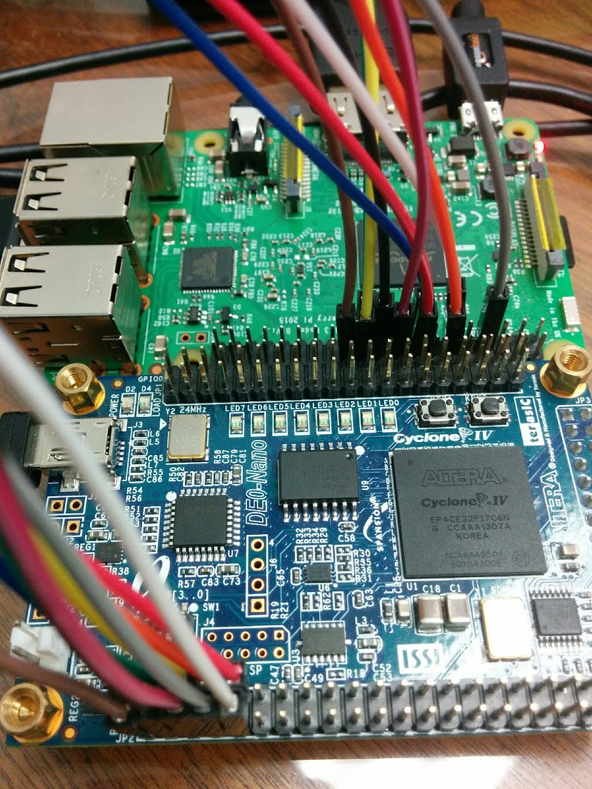
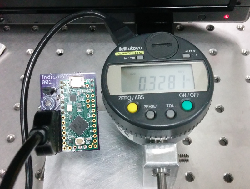
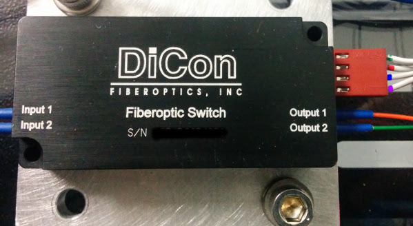
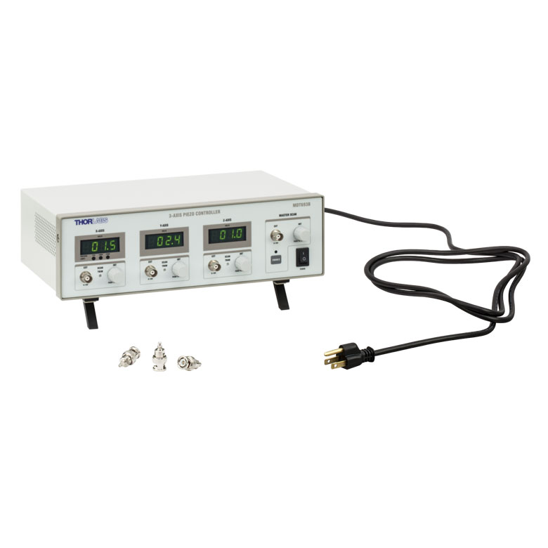
Now that I’ve (hopefully) convinced you that this is a good thing, I’ll go over adding an instrument to InstrumentKit. This tutorial is aimed at beginning python and git users, and will be aimed at creating an InstrumentKit driver for this lovely Thorlabs Piezo Controller:

Thorlabs MDT693B

Fork the InstrumentKit repository

Create a Github account, if you don’t already have one. Go to the InstrumentKit repository and click on the “Fork” button in the top right corner. If you have Windows, download Git for Windows. Open up git bash, go to a directory where you store your projects, and type:

git clone https://github.com/your_username/InstrumentKit
git checkout develop
git checkout -b thorlabs-mdt693B

To explain - first we created our own personal copy of the InstrumentKit repository (we forked it), then we made a copy on our computer (git clone), then checked out the development branch (checkout develop), and finally we made a branch off of the development branch (git checkout -b thorlabs-mdt693B).

The doc subdirectory in InstrumentKit contains instrument use examples; the instruments directory contains the source code. Within instruments, instruments are sorted into subdirectories by manufacturer. There are two additional folders - tests, which contains unit tests, which allow developers to check that changes to drivers do not change the operation of the device, and abstract_instruments, which contains generic code related to multiple devices. For example, for serial devices, it defines a generic SerialCommunicator device with query and command methods. Using an abstract instrument class allows you to avoid the most common ways that a serial communication protocol can be messed up.

Creating the Instrument

Create a new file under instruments->thorlabs called mdt693B.py.

InstrumentKit
└── instruments
    └── thorlabs
        ├── __init__.py
        ├── lcc25.py
        ├── _packets.py
        ├── pm100usb.py
        ├── sc10.py
        ├── tc200.py
        ├── thorlabsapt.py
	├── thorlabs_utils.py
        └── mdt693B.py

In mdt693B.py, start off by adding the bash path to python, then a comment declaring what the module is for:

#!/usr/bin/env python
# -*- coding: utf-8 -*-
"""
Provides the support for the Thorlabs MDT693B Piezo Controller.

Class originally contributed by Catherine Holloway.
"""

Next, like most python files, we need to import things. absolute_import and division are imported for python 2 to 3 compatibility. InstrumentKit uses the quantities library to handle unit conversion, but the convention is to import it as pq as most of the units are defined by single characters, so typing is minimal. For example, in this driver, we will be making use of pq.V. Our device is going to use the abstract_instrument Instrument as a template. We will also use the templates ProxyList, bool_property, int_property and unitful_property.

# IMPORTS #####################################################################

from __future__ import absolute_import
from __future__ import division

import quantities as pq

from instruments.abstract_instruments import Instrument
from instruments.util_fns import ProxyList, bool_property, int_property, \
    unitful_property

# CLASSES #####################################################################


class MDT693B(Instrument):
    """
    The MDT693B is is a controller for the voltage on precisely-controlled
    actuators. This model has three output voltages, and is primarily used to
    control stages in three dimensions.

    The user manual can be found here:
    https://www.thorlabs.com/drawings/f9c1d1abd428d849-AA2346ED-5056-1F02-43AE1247C3CAB43A/MDT694B-Manual.pdf
    """

The class keyword are like namespaces in Visual Basic or C#, or structs in C. This allows us to organize the attributes of devices in a logical way within a hierarchy. For example, we can imagine a multichannel voltage device being accessed like:

mc = MultichannelVoltageSupply()
mc.num_channels = 4
mc.channel[3].voltage = 3*pq.V
mc.channel[1].enable = True

the __init__ keyword is like a constructor on C++ classes - it gets called any time MDT693B() is called, and contains the code we want to run on initialization. Our device is based on the template Instrument, so in our intialization function, we need to call Super on it to make sure the Instrument gets initialized. Next, from the manual we can read that each query or command is terminated by a Carriage Return (\r) and Line Feed (\n) character, and that the device will print a prompt character when it is ready for new input. If we define these variables in our init, they will be passed up to Instrument when query or sendcmd are invoked, and will be handled appropriately. The variable self._channel_count is used to tell the ProxyList template that this device has three channels.

    def __init__(self, filelike):
        super(MDT693B, self).__init__(filelike)
        self.terminator = "\r\n"
        self.prompt = "> "
        self._channel_count = 3

In python, all class methods take self as the first word. self is like the this keyword in C++ or Java. The second argument to the initialization is a pointer to the active serial communication channel - it is created and sent to the MDT693B using the Instrument.open_serial method.

We’ve created the skeleton of our driver, now we need to add it to the file instruments/thorlabs/__init__.py so that it can be found once InstrumentKit is installed:

from .mdt693B import MDT693B

Now, we’ll be able to access our device from any python script as:

from instruments.thorlabs import MDT593B

Using Factories

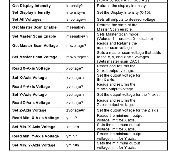
Now for the actual meat and potatoes of the driver. The commands are defined on page 18 of the User Manual.

mdt693b commands

One thing to notice is that the commands for all three channels are relatively similar. We can minimize our typing by creating a generic channel class within our MDT693B class:

    class Channel(object):
        """
        Class representing a channel on the MDT693B
        """

        __CHANNEL_NAMES = {
            0: 'x',
            1: 'y',
            2: 'z'
        }
        def __init__(self, mdt, idx):
            self._mdt = mdt
            self._idx = idx
            self._chan = self.__CHANNEL_NAMES[self._idx]

This initialization function is a bit more confusing - self._mdt is a link back up to the parent device, self._idx is the index value of the channel, and self._chan is a printable version of the channel name, which will be useful in generating the commands. From the manual, we can see that every channel has exactly three properties - the current set voltage, and the minimum and maximum allowable voltages. We would like to be able to set or get these variables as easily as you would any other independent variable, thus we should use the @property decorator. A getter/setter pair look like this:

        @property
        def voltage(self):
            """
            Gets/Sets the channel voltage.
            
            :param new_voltage: the new set voltage.
            :type new_voltage: quantities.V
            :return: The voltage of the channel.
            :rtype: quantities.V
            """
            return float(self._mdt.query(self._chan+"voltage?"))*pq.V
        
        @voltage.setter
        def voltage(self, new_voltage):
            new_voltage = new_voltage.rescale('V').magnitude
            self._mdt.sendcmd(self._chan+"voltage="+str(new_voltage))

This code may look confusing or pointless for those unfamiliar with object-oriented programming, but it will be invaluable once you’re used to it. It allows us to do things like:

print(mdt.channel[0].voltage.rescale('mV')

or

mdt.channel[0].voltage = my_joules/my_current

The first method of this pair, under the @property decorator, tells the parent device to send the query “xvoltage?” (if on channel 0, for example), convert the resulting string to a float, then assign its units as volts.

The second method of this pair, under the @voltage.setter decorator, re-scales the input value to volts, then sends the command “xvoltage=10” (if the new value was 10 V) to the device.

The same getter/setter pairs are copied for the minimum and maximum voltages.

In order to tell the MDT693B device that that channels 0-2 point to a voltage channels with the labels ‘x’, ‘y’ and ‘z’, we need to add a channel property that calls the ProxyList template:

    @property
    def channel(self):
        """
        Gets a specific channel object. The desired channel is specified like
        one would access a list.

        :rtype: `MDT693B.Channel`
        """
        return ProxyList(self, MDT693B.Channel, range(self._channel_count))

The rest of the properties defined in the manual follow a common pattern, so we can use existing templates (also sometimes called factories) in InstrumentKit to define them.

For example, enabling/disabling the master scan function is a prime target for a boolean property, since it has only two values:

    master_scan_enable = bool_property(
        "msenable",
        "1",
        "0",
        doc="""
        Gets/Sets the master scan enabled status.

        Returns `True` if master scan is enabled, and `False` otherwise.

        :rtype: `bool`
        """,
        set_fmt='{}={}'
    )

Here, we use the first three values to declare the property keyword, then the values returned by the device for enabled and disabled. The set_fmt variable is used to define the format for the commands.

The display screen brightness is a unitless property, thus we can use the int_property to generate it:

    intensity = int_property(
        "intensity",
        valid_set=range(0, 15),
        set_fmt="{}={}",
        doc="""
        Gets/sets the screen brightness.

        Value within [0, 15]

        :return: the gain (in nnn)
        :type: `int`
        """
    )

The manual defines the valid range of values for intensity as being between 0-15. If it gets something outside of that range, it will likely behave oddly or report an error message, which will mess up serial communication. If we use this template, we can catch these out-of-bound errors before they get set to the device.

Finally, to show off another template, consider the master scan increment voltage. It is a unitful property - the value returned by the device is in volts, rather than the unitless integer setting for the screen brightness intensity. Here, a unitful_property template can be used:

    master_scan_voltage = unitful_property(
        "msvoltage",
        units=pq.V,
        set_fmt="{}={}",
        doc="""
        Gets/sets the master scan voltage increment.

        :return: The master scan voltage increment
        :units: Voltage
        :type: `~quantities.V`
        """
    ) 

It is the same as the two previous templates, except with the units variable set to volts to declare that the master_scan_voltage is in volts.

Creating an Example Script

Now that you’ve finished your driver, a sample script should be included so that others know how to use your device. Sample scripts are stored under doc/examples and then sorted by manufacturer:

InstrumentKit
└── doc
    └── examples
        └── thorlabs
            └── ex_mdt693b.py

ex_mdt693b.py looks like this:

"""
An example script for interacting with the thorlabs MDT693B piezo driver.
"""
import quantities as pq
from instruments.thorlabs import MDT693B

mdt = MDT693B.open_serial(vid=1027, pid=24577, baud=115200)

for i in range(0, 3):
    print("The voltage on ", i, " is ", mdt.channel[i].voltage)
    print("The minimum on ", i, " is ", mdt.channel[i].minimum)
    print("The maximum on ", i, " is ", mdt.channel[i].maximum)

mdt.master_scan_voltage = 1*pq.V
mdt.master_scan_enable = True

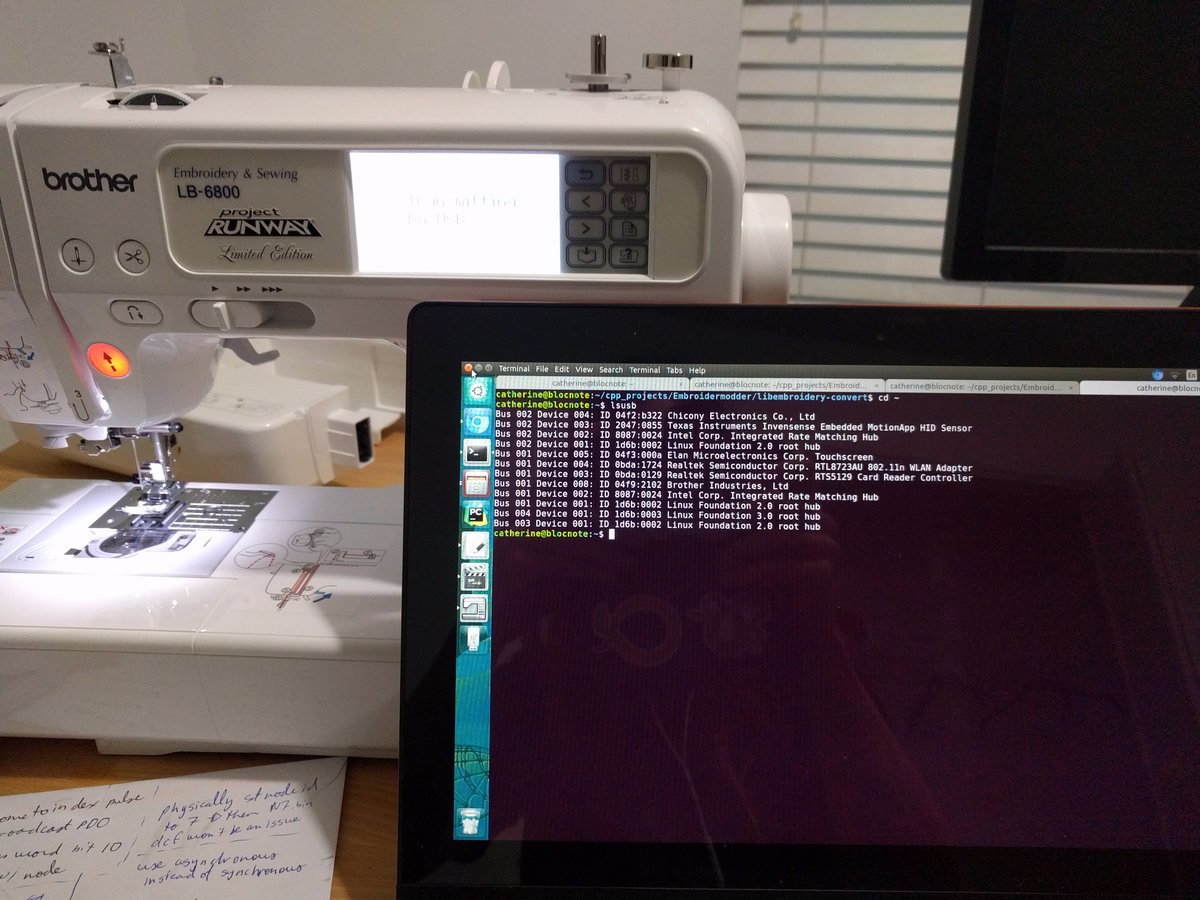
Although the method open_serial can be called by specifying a port, such as COM8 or /dev/ttyUSB0, it can also be specified using the device’s vid, pid, and optional serial number. As assigned ports can change hap-hazardly based on the order in which devices are plugged into the computer, or at the whims of the operating system, it is often preferable to open the serial connection with the vid/ pid pairs instead of the port. These IDs can be determined either by opening the port’s preferences under the device manager on Windows, or with the command lsusb in Linux.

If you have multiple devices with the same product and vendor ids, you can differentiate them by the optional variable serial_number, i.e.:

hardware1 = Device.open_serial(vid=1027, pid=24577, serial_number="aaaaaaaaa", baud=9600)
hardware2 = Device.open_serial(vid=1027, pid=24577, serial_number="aaaaaaaab", baud=9600)

The sample code opens a serial connection on this port and passes it to the MDT693B class for initialization. Then, it prints the voltage values for the three channels, then sets the master_scan_voltage and finally enables the master scan.

Contributing Back

Once your driver is finished, you should write unit tests for it, but that is enough material for another post. To contribute the device back to the community, stage your changes for a commit. In git bash, type the following:

cd InstrumentKit
git add instruments/thorlabs/__init__.py
git add instruments/thorlabs/mdt693b.py
git add doc/examples/thorlabs/ex_mdt693b.py
git commit -m "added MDT693B driver"
git push origin thorlabs-mdt693B

We changed directory into InstrumentKit, then added the three files we changed to the repository, then created a commit with the message added MDT693B driver, then pushed it to our github repository with the branch name thorlabs-mdt693B.

Once that is branch is public on github.com, we can create a pull request on github.com/Galvant/InstrumentKit. This allows the original developers of InstrumentKit to look over and approve our code. Hopefully the changes will be minimal, and your new driver will be available to others!

08 August 2016

IV - BadBadNotGood

IV - BADBADNOTGOOD

Toronto Jazz trio BadBadNotGood are now a quartet, having invited saxophonist Leland Whitty, the secret sauce behind the band’s best previous output, Confessions, to join as a full member. I’m not a fan of Ghostface Killah’s style of barking unrhythmic style of rapping, so their collaboration album Sour Soul was a let down, but their latest album IV is a return to their old style, matured. It’s their best release yet.

Chompy’s Paradise is devine. The grove is smooth and hypnotic broken up with progressive rhythm changes and a chorus that slowly ascends to heaven. Another highlight is IV, with fast, dueling bass, piano and saxophone lines that suddently become soft and sweet.

This album is not totally flawless. The tone of Colin Stetson’s saxophone playing on the song Confessions Pt II is a little too harsh for my taste. The organ on Time Moves Slow clashes with the vocal melody.

Still, the album on a whole is a fantastic. The band continues to progress towards a sound that fully-absorbed jazz fans will find enthralling while seemlessly blending with contemporary hip-hop, as with the song Hyssop of Love.

Monomania, Vision Crimes and Self-titled Split EPS - Child Bite

Monomania - Child Bite Vision Crimes - Child Bite Child Bite / We Are Hex Split EP - Child Bite

Aside from missing friends, my biggest regret about moving to San Diego was missing Vektor open for Voivod in Toronto. Though I may have missed that concert, I instead was able to see them when the played San Diego, where they were opened by Child Bite. Following their frenetic but fantastic live performance, I bought their three EPs on Bandcamp, Monomania, Vision Crimes and their self-titled EP.

It’s hard to define Child Bite’s genre. Like Voivod, they are closest to punk rock, but with lyrics like Can or Zappa combined with some sludge metal sounds over a mid-century musical melody. Many songs start off with rough production or a punk-like simplicity to the singing and melody. The melodies on certain songs, like Wrong Flesh, are annoying in their simplicity and lack of resolution. I’m not sure if this is intentional. A minute into most songs, however, and it has progressed into unexpected territory. It’s this progression and a lot of technical talent that have kept my attention.

Wriggle - Clipping.

Wriggle - clipping.

Clipping. is a experimental noise-rap group fronted by Hamilton start Daveed Diggs. Often compared to Death Grips, their comparison ends at the outlandishness of the composition. Unlike Death Grips, the Diggs aims to tell coherent and descriptive stories that put you in the mind of someone else with the drama and clarity expected of a Shakespearean actor. It’s this rap storytelling that made me fall in love with their last albums Midcity and CLPPNG, especially the songs Story and Summertime. The have now released an EP to tease their next album, Splendor & Misery which comes out next month.

The EP begins with Shooter, a song describing three different types of violent people in our modern society. It’s an interesting concept, but the entire song being written in hashtag rap, which I can’t listen to without thinking of Iggy Azalea’s line “Watch a new Kardash, call me Kylie”.

Back Up features the clipping triumvirate of sound effects for the bassline and percussion, detailed descriptions of environments, and sarcastic protrayals of hardcore drug users.

Wriggle is interesting because it’s a song about BDSM peppered with moments of trepidation, not merely bragging about sex or talking about how attractive/horny his partner is. The chorus and composition are equally frenetic and odd.

Hot Fuck, by contrast is a generic sex song who’s sole novelty is that it speeds up near the end like a climax.

The last song on the album is a bit of a snoozer. The singing is bad.

Although three of the songs are merely alright, the two fantastic songs, Back Up and Wriggle are well worth the price of the EP. I look forward to the album next month.

07 August 2016

I went to the Euro Python conference in Bilbao, Spain, directly from SciPy on July 17th. Though severely jet-lagged and with a head full of stuff from SciPy, I enjoyed Euro Python immensely. Bilbao is a lovely (and cheap) city, and I’m glad I had an excuse to visit. Here are my favourite presentations from Euro Python.

I also had another opportunity to speak about pyglet helper, but it was near identical to my SciPy presentation.

Python at the European Gravitational Observatory

Elena Cuoco - Python in Gravitational Waves Research Communities

Wednesday’s keynote was given by Jameson Rollins of LIGO, and while it was good, as a physicist I got more out of Elena Cuoco’s talk the day before. While Rollins’ keynote was devoted mostly to explaining gravitational waves and their detection to a broad audience, Cuoco dove right into the tools used in the gravitational waves research communities. While most of it, such as the pyrap library for radio astronomy data processing and the pycbc library for studying compact binary coalescence (black holes orbiting each other), do not apply to optical quantum computing, the pykat library for simulating interferometers is. The performance of the entangled photon sources I help design depends on how well an optical interferometer can be stabilized, and I find simulation helpful. Who knows, perhaps the intensive effort that the gravitational wave community has put into clearing up and analyzing optical data can also be helpful in future.

Go and Python Side-by-Side

Max Tepkeev - Do I need to switch to Go(lang) ?

Earlier this year I dipped my toes into the Go language in order to fix some bugs in the arduino builder, and while I managed to fix what I wanted to fix, I was confused by many things in the Go language that introductory presentations on youtube did not clarify. Max Tepkeev’s talk introducing Go was exactly what I needed - in addition to placing Go in relation to other languages and describing some use cases, his presentation features several slides of side-by-side python and go examples. I would highly recommend this presentation to any pythonistas going to Go.

Live OpenGL with Python

Roberto De Ioris - Modern OpenGL with Python

Roberto De Ioris teaches computer graphics at an Italian Video Game academy, and gave an hour-long tutorial on the basics of OpenGL using the python bindings. Though a lot of it was stuff you could speed through in a tutorial, De Ioris is a good teacher and the demos brought the material to life. I also appreciated hearing his thoughts on the stability and usability of Vulkan and clarify the difference between various shader and lighting techniques.

The Scientist and the Web Developer should be Friends

Gaël Varoquaux - Scientist meets web dev: how Python became the language of data

In undergrad I worked part-time as a web developer. The skills I picked up there transferred to my summer research projects in bioinformatics, but once I got to grad school, (for experimental physics), my skills were treated as useless. If only I could have made my point as eloquently as Gael Varoquax did in his keynote, perhaps I could have convinced my fellow physicists that databases were good and useful. It’s also a great lecture as it explains the background of scientific computing and some of numpy’s internals.

Teaching a Computer to Love (or at least when someone else loves something)

Katharine Jarmul - I Hate You, NLP... ;)

I regret missing seeing this in person - there was a talk on algorithmic trading using python, and I’ve read one too many Michael Lewis books lately. The algorithmic trading talks was boring - it was a stealth recruitment pitch for a trading company, and with no tutorials on either stock trading or pricing. Katharine Jarmul’s talk on using machine learning and natural language processing to determine the emotional intention of human text, such as tweets. It was good because it covered bleeding-edge research with the aim of helping mere programmers build stuff.

02 August 2016

I am grateful that writing critiques of the music people recommend to me has not discouraged new recommendations. I enjoy listening to everything once, so please continue to send me stuff! Here are my thoughts on the recommendations I’ve listened to recently.

Sleep

I introduced John to stoner/sludge metal band High on Fire, he returned the favor by digging through frontman Matt Pike’s discography and introducing me to Sleep. Sleep’s sound is on the rougher and distorted side of sludge metal, sounding more like Sourvein’s latest than High on Fire. It makes sense, since Sleep was active a decade before its predecessor, but it is interesting that Pike went for a faster and less distorted sound with High on Fire, whereas other stoner metal bands have progressed to slower and more distorted sounds. Perhaps the popularity of bands like Baroness and High on Fire have led to a newfound appreciation to 90’s stoner metal.

The first two albums, Volume 1 and Holy Mountain have some good tracks, including my favourite, the gut punching and hypnotic Dragonaut, however, the real masterpiece of their discography is Dopesmoker, a churning bible-themed epic about the genre’s favourite substance. The track is occasionally repetitive, but there are frequent fantastic guitar licks that keep the track/album interesting for over an hour.

Katatonia

Several months ago Jeff sent me a link to the latest singles off of Swedish death metal now progressive rock band Katatonia’s latest album, The Fall of Hearts. Though I wasn’t enamoured with the tracks, I decided to listen to the rest of their discography.

Their early 90s death metal albums, Dance of December Souls and Brave Murder Day, are listenable, but they’re not as interesting as more contemporary bands in the same genre, who utilize a greater range of tempos and chords progressions. I would describe these albums as chamber music played in a death metal style.

In the late 90s their style changed dramatically to more gothic, melancholy sounds with clean pop-like vocals. Renske’s voice was not quite suited to this style on their first release after the change, Discouraged Ones, but his voice improved with time. The live versions of the songs off of Discouraged Ones on last year’s Sanctitude are a great improvement. The consistency of style and quality was cemented on their follow up Last Fair Deal Gone Down.

Viva Emptiness has several songs that annoy me - Omerta has an interesting style but no instrumental break or progression, the lyrics on Criminals make no sense and do not fit the intensity of the bass line. As the theme of the album is depression, perhaps these faults are intentional - a sufferer of depression is unlikely to feel a large spectrum of emotions, and when they do it is unlikely to make sense in context. Intentional or not, it doesn’t make for a pleasant listening experience.

On their most recent albums, The Great Cold Distance, Night is the New Day, and Dead End Kings, Katatonia are the Alicia Keys of prog-metal: pleasant to listen to, but the singing is weak and the songs never go anywhere. Chelsea Wolfe is an example of this slow, moody metal-flavoured singing of this style that I find very captivating. By contrast, this sounds like some Nu-Metal band took an ambien.

The Moody Blues

After confessing my love of 70s prog metal to my dad, he confessed that he’d been teased in his early 20s for liking The Moody Blues. I had listened to The Magnificent Moodies during my teenage Beatles-led British 60s pop music phase, so it hadn’t occured to me that they were proggy. But their psychadelic, symphonic rock Days of Future Passed is sometimes considered the first prog album.

Their albums of the late 60s/early 70s combine the classical symphonic and movie soundtrack sounds that ELP and Yes were adapting with the soft harmonic singing over strings of folk acts like Simon and Garfunkel. Though the composition and technique on these albums are great, the lyrics aren’t. Some of their songs remind me of Eve of Destruction - the heaviness of the subject matter was assumed to carry the song.

The highlight of their discography are the three albums released with former keyboardist Patrick Moraz, Long Distance Voyager, The Present and The Other Side of Life. These albums have, unsurprisingly, the great piano composition and emotional range reminiscent of a Yes album.

However, after Moraz left, the quality fell steeply off as they chased modern synthpop styles in order to relive their early 80s success. It’s more obviously synthetic and unpolished than the worst things Asia put out in the 90s. Like Asia they also put out unlistenable Christmas songs. At least Asia had enough sense not to bother with techno.

My recommendation - everything between ‘68 and ‘86 is great, the rest is unlistenable.

23 July 2016

The SciPy 2016 conference was last week in Austin, Texas. Despite the suffocating heat, I got to visit the Lyndon B Johnson Presidential Library, see Ghostbusters in the Alamo Drafthouse, and sleep in an airstream trailer in someone’s back yard. More importantly, I had the opportunity to talk about pyglet_helper, and learn a lot of useful things about python. Here are a few personal highlights.

Making Python Packages for Windows is Hard

Frequent visitors to PyPI may have noticed that many common packages have recently switched to using wheels. No longer will we twiddle our thumbs restlessly as we watch setup.py install churn through line after line of gcc warnings! That is due to the excellent efforts of Nathaniel Smith, who spoke about his work:

Reinventing the .whl

Wheels can be built for several different versions of python using a provided docker image. The Numpy and Scipy builds are built with OpenBLAS, which is an exciting development. Smith seems confident that it will be possible to bundle OpenBLAS with Numpy wheels on Windows soon as well, which will be a big time-saver for me.

At 9:12, he describes exactly what is needed to easily compile wheels for Windows - the lack of a good compiler. This was brought up by an audience member at the python core developers panel at Euro Python a few days ago and the panellists seemed surprised. I think the problem is that the people with the domain knowledge of compilers are exclusively linux users and windows users would prefer to use Anaconda. In between are a few like me, who both need to use Windows for device drivers but also want to use obscure packages in PyPI, without fussing with the visual studio compiler.

Linting Text

As much joy as writing this blog has been, it has forced me to confront the fact that I am not a good writer and I should be better at editing my text. I acquired an appreciation for style guides from the one journalism class I took in undergrad, but 10 years later I’ve forgotten most of the rules. Thus, I am keenly interested in Michael Pacer and Jordan Suchow’s project, proselint:

A linter for prose

I’ve tried it out for myself on my blog posts, and at the moment it has difficulty with markdown, especially in accidentally prose-linting code blocks. Regular expressions have only a limited ability to fix bad writing, but I will take all the help I can get. I’m interested in building a PyCharm extension for proselint and in incorporating proselint into my githubio build process. I’m not sure how successful I will be in my current set-up, as my build uses ruby.

EPIC Async

Though I have been working in experimental physics for the past six years, I had never heard of the Experimental Physics and Industrial Control System (EPICS) until Daniel Allen’s talk. I work on experiments with only up to one control computer at a time, whereas EPICS is used big, hundred-party experiments such as Synchrotrons or LIGO. From a conceptual level, it reminds me of the Robotics Operating System, with its publishers and subscribers. In his talk, Allan describes an experimentalists’ dream: capture your data along with the operations in a retrievable format, and have a system that can roll back to a recoverable state if something goes wrong.

Experiments as Iterators

These are design goals for my projects as well, even if they only have 3 users. I have limited time with my equipment as well, and needing to repeat an experiment because some metadata was missing is a waste. I don’t quite understand the usage of asyncio in this context, but I’m eager to learn how it could benefit my experimental automation.

Imputation is Important for the Real World

John’s recently defended PhD thesis is about applying machine learning techniques to filling missing data (imputation) on incomplete ranked ballots in order to maximize the fairness of elections. Imputation is an important consideration when applying algorithms to data in the real world, as Deborah Hanus demonstrated in her talk, featuring her work with optimizing the treatments for HIV patients:

Dealing with Missing Data

Due to issues surrounding shift work and childcare, transportation access, or human error, HIV patients sometimes miss their regularly scheduled blood tests. Imputation allows the machine learning algorithm to predict optimal dosages even in the presence of missing data. Aside from being interesting research, the talk also provides a good layman’s explanation of imputing random walks over time.

12 July 2016

High Finesse is a German optics company that makes high-quality spectrometers and wavelength meters. I’ve written a python interface to their provided wlmData driver in order to grab spectrum data off a LSA UV Vis 2, however, it is likely to work with other spectrometers and wavelength meters that use the same library. Unfortunately, at this time High Finesse only provides windows drivers.

Installation

To install this library, use:

git clone https://github.com/CatherineH/pyHighFinesse
cd pyHighFinesse
python setup.py install

The project will soon be available on pypi as pyHighFinesse.

Example Script

The following minimal script grabs and plots the spectrum dataframe

from lsa import Spectrometer
import matplotlib.pyplot as plt
reading = Spectrometer()
spectrumdata = reading.spectrum
spectrum = spectrumdata.set_index('wavelength')
_ax = spectrum.plot()
_ax.legend_.remove()
_ax.set_title('LSA Analysis output')
_ax.set_xlabel('Wavelength (nm)')
_ax.set_ylabel('Intensity')
plt.show()

spectrum Screenshot

The WLM and LSA

High Finesse provides a dynamic library called wlmData.dll, which is installed to the system32 directory. They also provide a C header called wlmData.h which contains additional constants useful to the interface such as error codes and options.

The LSA is a GUI that also a server process that communicates with the instrument. The python interface communicates and shares memory with the LSA through the dynamic library. The python interface needs to start up the LSA in order to get data off the spectrometer.

Parsing the Header file

The header file contains a lot of useful information about error codes, return types and options. In future, the function return type could be used to automatically populate the ctypes restype value, but for now only error codes and options are red in.

The constants section of the header file is deliminated by a line-long comment that contains the word “Constants”, so parsing begins after that line is encountered

begin_read = False
for line in f_in.readlines():
    if line.find("Constants") > 0:
        begin_read = True

Next, if a line contains the keywords const int, the line probably contains a useful value to parse. The keywords, whitespace characters and semicolon are removed, and the string is split around the equals sign

    if begin_read and line.find("const int") > 0:
        values = line.split("const int")[1].replace(";", "") \
                     .replace("\t", "").replace("\n", "") \
                     .split("//")[0].split(" = ")

Header values are added as attributes to the Spectrometer object. The values of the integer constants are one of three things: a number, a string representing a previously declared integer constant, or an expression adding previous constants and numbers. Since there is no built-in function to check whether a string can be parsed as an integer, this parsing is done as a nested try/catch block. First the string is parsed as an int; if that fails, it is split around the plus sign. (The header expressions currently only contain additions). Then, there must be a second integer check, and if that fails, it assumes that the string is a value that python has previously parsed in.

        try:
            # first, attempt to parse as int
            setattr(self, values[0], int(values[1], 0))
        except ValueError:
            parts = values[1].split(" + ")
            # if that fails, parse as a value
            value = 0
            for part in parts:
                try:
                    value += int(part, 0)
                except ValueError:
                    value += getattr(self, part)
            setattr(self, values[0], value)

Errors should be added to their corresponding sets for future error checking. Constants starting with Err occur when measurement values or settings are read from the LSA; constants starting with ResErr occur when settings are changed in the LSA. The list of ResErr errors contains an error 0 for NoErr to confirm that the setting was changed, this error is purposely excluded fro m the list of errors.

        if values[0].find("Err") == 0:
            if 'read' not in self.errors_list.keys():
                self.errors_list['read'] = []
            self.errors_list['read'].append(values[0])
        if values[0].find("ResERR") == 0:
            if 'set' not in self.errors_list.keys():
                self.errors_list['set'] = []
            # no not append the "NoErr" Error
            if getattr(self, values[0]) != 0:
                self.errors_list['set'].append(values[0])

Finally, the wavelength ranges are also defined in the header, however these do not appear to correlate with the actual values in the LSA. For the moment, this is hard-coded for the observed values. If you have a High Finesse device other than an LSA, please let me know what these ranges are for you.

        self.wavelength_ranges = [(0, (190, 260)), (1, (250, 330)),
                                  (2, (320, 420))]

Accessing Memory

The functions in the WLM dynamic library will either return a value, such as a short, long or double, or an address in memory. The return type must be specified in order for the output to be read correctly.

For example, c_double must be specified when reading floating point numbers, such as temperature or wavelength:

get_wavelength = self.lib.GetWavelength
get_wavelength.restype = c_double
wavelength = get_wavelength(0)       

Other entries, such as GetPattern or GetAnalysis will return an address in memory of an array of numbers. The number of numbers can be queried using the GetAnalysisItemCount, the size of the numbers in bytes can be queried using GetAnalysisItemSize: 2 for c_short 4 for c_long and 8 for c_double. To remove redundant code, all three values are queried using the same lines of code by looping over the parameters for each of the x and y axes of the analysis pattern:

results = {}
parts = [{'wavelength': 'X', 'intensity': 'Y'},
         {'size': 'ItemSize', 'count': 'ItemCount', 'address': ''}]
for axis in parts[0]:
    results[axis] = {}
    for value in parts[1]:
        getter = getattr(self.lib, 'GetAnalysis'+parts[1][value])
        getter.restype = c_long
        component_arg = getattr(self, 'cSignalAnalysis'+parts[0][axis])
        results[axis][value] = getter(component_arg)

These values can then be read in using the cast function:

DATATYPE_MAP = {2: c_int, 4: c_long, 8: c_double}
...
memory_values = {}
for axis in parts[0]:
    access_size = DATATYPE_MAP[results[axis]['size']]*results[axis]['count']
    memory_values[axis] = cast(results[axis]['address'],
                               POINTER(access_size))

Finally, the individual numbers in the array can be accessed using the contents property. For ease of use in analysis, the values are then stored in a pandas dataframe:

spectrum_list = []
for i in range(0, results['wavelength']['count']):
    spectrum_list.append({'wavelength': memory_values['wavelength'].contents[i],
                          'intensity': memory_values['intensity'].contents[i]})
spectrum = DataFrame(spectrum_list)

LSA Oddities

The WLM driver occasionally behaves in ways that contradict the user manual. For example:

  • Hiding the WLM control does not also hide the long term analysis window
  • The wavelength ranges provided in the header do not correspond to the actual wavelength ranges on the instrument
  • The parameters for wide and precise spectrometer analysis appear to be reversed.

It is likely that other High Finesse devices also exhibit odd behavior, however this module was currently tested with an LSA UV Vis 2. If this module results in odd behavior on your device, please let me know by submitting an issue on github.

07 July 2016

I stumbled over some fairly obvious things when importing a Windows dll in python this morning. I’m writing this post to shorten the amount of time I spend reading Stack Overflow next time.

The code I will be using for this post is:

from ctypes import cdll
lib = cdll.LoadLibrary("mydll.dll")

Are you using the static version of the library instead of the dynamic version?

ctypes can only import dynamic libraries. If you attempt to load a static library, you will get the error:

  File "Python35\Lib\ctypes\__init__.py", line 425, in LoadLibrary
    return self._dlltype(name)
  File "Python35\Lib\ctypes\__init__.py", line 347, in __init__
    self._handle = _dlopen(self._name, mode)
OSError: [WinError 193] %1 is not a valid Win32 application

Make sure the dynamic .dll file is loaded, not the static .lib file. If only static libraries are provided, it might be possible to recompile as a dynamic library, but I did not try this.

Are you using 32 bit python with a 64 bit library?

Using a 64-bit dll with 32 bit python results in the error:

   File "Python35\lib\ctypes\__init__.py", line 429, in LoadLibrary
    return self._dlltype(name)
  File "Python35\lib\ctypes\__init__.py", line 351, in __init__
    self._handle = _dlopen(self._name, mode)
OSError: [WinError 193] %1 is not a valid Win32 application

To solve this, download the Windows x86-64 version of python, and configure your IDE to use this python interpreter.

Are you using the 32 bit version of ctypes with a 64 bit version of python?

If you install the 64 bit version of python alongside the 32 bit version, it is likely that your environment variables will still be set up to point the PYTHONPATH to the 32 bit versions of the python libraries.

This will result in the error:

   File "example.py", line 1, in <module>
    from ctypes import cdll
  File "Python35\lib\ctypes\__init__.py", line 7, in <module>
    from _ctypes import Union, Structure, Array
ImportError: DLL load failed: %1 is not a valid Win32 application.

To fix this, I set the PYTHONPATH in my IDE to be Python35\Lib\;Python35\libs; Python35\DLLs

On Windows, with python > 3.5, it is important to add the DLL folder; the _ctypes module lives in there now.

07 June 2016

My research group in grad school had an unfortunate culture of stealing equipment from other people’s experiments when they weren’t around. I participated in this culture as well, but I tried to replace the things I took before they returned. However, this did not spare me from the ire of a Postdoc1 who pointed out that windows assigns device names by serial number, thus my replacing a power meter with an identical copy had caused him an hour of debugging time until he opened up the device manager.

Later, out of grad school and working on robots with even more hardware, I discovered the joy of writing udev rules and spared myself many hours of plugging in usb cables to see what they enumerate as.

I’m now out of robotics and back in experimental physics. Most experimental physicists aren’t linux users, so a lot of scientific equipment is sold with drivers which are only functional on Windows.

I had reverted back to plugging and unplugging cables, until the other experimental physicist at work switched out the hardware in my experimental setup overnight. After I had calmed down, decided to find another way.

Here’s my solution. PySerial has a lovely tool called list_ports which will list a bunch of handy information about the available com ports. By matching the vendor and product IDs, (or in the case of devices that both use the FTDI FT232R chip, also the serial number) I can guess the devices:

from serial import Serial
from serial.tools import list_ports

# hardware is represented as a tuple of (vid, pid, serial_number (if needed), baud_rate)
HARDWARE = {'temperature_controller': (1027, 24577, 'serial1', 115200),
            'counter': (1027, 24577, 'serial2', 19200),
            'motor_controller': (5824, 1155, 9600),
            'laser': (10682, 2, 115200)}

def map_hardware():
    com_ports = dict()
    for key, value in HARDWARE.items():
        found_port = False
        for port in list_ports.comports():
            if len(value) > 3:
                if port.vid == value[0] and port.pid == value[1] and port.serial_number == value[2]:
                   found_port = True
                   com_ports[key] = port.device
                   break
            else:
                if port.vid == value[0] and port.pid == value[1]:
                   found_port = True
                   com_ports[key] = port.device
                   break
        if not found_port:
            raise RuntimeError("device matching ids for key: ", key, " not found")
    return com_ports

ports = map_hardware()
handles = dict()

for key in ports.keys():
    handles[key] = Serial(ports[key], HARDWARE[key][-1])

This is a simplification. I import modules from InstrumentKit to do the actual communication rather than writing the commands directly to the handles.

  1. Brendon, if you’re reading, I’m still sorry about this. 

24 May 2016

Seaborn is a wonderful python package for creating statistical plots like those found in R. Although the documentation and API does not expose much, the modules are built on top of matplotlib, a versatile plotting library. Matplotlib has an incredible amount of customization, if you’re willing to dig far enough. My goal with this post is simply to document the customizations I have encountered. The changes are made on the ‘iris’ demo.

Empty Axes

Using seaborn with the default ubuntu matplotlib package (python-matplotlib) will result in plots with empty axes:

empty axes example

To resolve this, matplotlib must be updated past version 1.3:

$ sudo apt-get install libfreetype6-dev
$ sudo pip install --upgrade matplotlib

Custom Data Labels

Seaborn will take the keys from the dataframe as the x and y axes labels, and assign labels only if the subplots are around the left and bottom sides of the grid. Replacing them means dipping down to the axes level:

import seaborn as sns; sns.set(style="ticks", color_codes=True)
iris = sns.load_dataset("iris")
g = sns.pairplot(iris, hue='species')
replacements = {'sepal_length': r'$\alpha$', 'sepal_width': 'sepal',
                'petal_length': r'$\beta$', 'petal_width': 'petal',
                'versicolor': 'bloop'}

for i in range(4):
    for j in range(4):
        xlabel = g.axes[i][j].get_xlabel()
        ylabel = g.axes[i][j].get_ylabel()
        if xlabel in replacements.keys():
            g.axes[i][j].set_xlabel(replacements[xlabel])
        if ylabel in replacements.keys():
            g.axes[i][j].set_ylabel(replacements[ylabel])

Similarly, the hue categories are taken from the values in the dataframe. Most of the template graphs (such as pairplot), add a legend to the top level figure on being called, and this makes it difficult to edit.

In addition, the matplotlib Figure object does not provide a get_legend() method. Instead, it is possible to access via get_children(). The legend is the last artist added, so it will be at index -1:

for i in range(len(g.fig.get_children()[-1].texts)):
    label = g.fig.get_children()[-1].texts[i].get_text()
    if label in replacements.keys():
        g.fig.get_children()[-1].texts[i].set_text(replacements[label])

This is the resulting graph:

renaming labels example

Moving the Legend

There are plenty of ways to place a legend in a figure when it is created, but moving the legend once it is already in the figure is a different story. The one method I’ve found is to move the legend’s anchor using set_bbox_to_anchor. These numbers seem to be expressed as a function of the size of the total figure, and are expressed as (left, bottom, width, height) . Since the figure expands to fill the required space of all the artists, width and height can be zero. So, the following code will put the legend in the middle in the y direction but over right edge of the figure:

g.fig.get_children()[-1].set_bbox_to_anchor((1.1, 0.5, 0, 0))

moved legend example

20 May 2016

This month I bought three fantastic albums an an EP on my favourite DRM-free platform:

Sunburst - Fragments of Creation

Sunburst - Fragments of Creation

I am aware of only three things that my husband loves that I think are worse than subterranean trash fires: Slaughterhouse Five, Jupiter Ascending, and Dream Theater’s latest album, The Astonishing. I love Dream Theater, and think that their other two albums since Portnoy’s departure rank just under Images and Words, but listening to The Astonishing gave me DT fatigue. So I was hesitant to listen to Fragments of Creation by Sunburst when I read that it was marketed as an album for DT fans.

Fragments of Creation was worth waking up for - it’s like the frenetic playing of Fleshgod Apocalypse with triumphant DT melodies, guitar work and Labrie’s singing style. There are quite a few other progressive and metal influences: the fast synthesizer arpeggios that sound like songs off Asia’s Aura, TesseracT djent, and Rhapsody of Fire choral breaks. There are still some fresh ideas - I really like the xylophones in the background.

The singing often verges on Celine Dion-level corniness with all of the tremolos, or descends into Disturbed whining. The lyrics aren’t worth paying attention to: a lot of it is generic nu-metal stuff about pain and abandonment. The key change in Lullaby attempts to keep a song that had already expressed all of its ideas going for another 30 seconds. Finally, the playing isn’t quite tight, but the songs are fun enough that it doesn’t detract from the whole product.

The album is not perfect, but it is a much better DT album than DT’s last. Ravenskill who?

Vektor - Terminal Redux

Vektor - Terminal Redux

Vektor, the band that made me a thrash-metal convert, released Terminal Redux, a gothic space-opera concept album. It is as technical, ferocious and fascinating as their last two albums, but the addition of a cohesive storyline makes this album special.

The story is about some unspeakable evil plotting revenge on the civilization that punished it for previous crimes. Like the last Ghost album, several tracks have gospel choir singing in a positive key about the reincarnation of this great evil, which is utterly delightful. Vektor venture into slower territory on Collapse, which don’t quite hold my attention at slower speeds, though the interaction between counter melodies are still interesting.

Collapse is the one weak song on a substantial album.

Bent Knee - Say So

Bent Knee - Say So

Say So is a more pop, accessible, and fantastic sequel to Bent Knee’s 2014 album Shiny Eyed Babies. Although Bent Knee are called art-rock, I think of them as more like progressive pop/jazz music. The lead singer Courtney Swain can channel powerful Chanson emotions like Edith Piaf, but with all of the avant-garde, modern flourishes of a singer like Kimbra. The album starts off with a deeply unsettling song reminiscent of Shiny Eyed Babies’ Way Too Long, about foreign liquids covering or flowing uncontrollably out of your body, except this time tar instead of oil and toxic gas, then delves into female-centric themes. There are songs about the pre-pubescent angst of female childhood: I think the song Leak Water is about feeling like one of the peeing dolls that were popular in the 90s and the song Counsellor evokes memories of the emotional distance and bullying of my childhood peers. Other songs cover dissatisfaction with domestic life; lyrics on multiple songs mention dreaming of love and adventure while doing mundane things like driving kids around. Commercial and Good Girl are deeply sympathetic feminist anthems that should show Meghan Trainor and Jennifer Lopez how it’s done.

This album should be taken as a blueprint for a modern pop masterpiece - the songs can make you feel as excited as a Carly Rae Jepsen song, but the lyrics are as clever as something written by Sloan. This album combines the melancholy plaints of Melanie Martinez with the experimentation of Zappa, and the end result is simply flawless.

If nothing else, the album is worth it to hear a sung five-note arpeggio of the word hyperloop.

Gorguts - Pleiades’ Dust

Gorguts - Pleiades’ Dust

All your favourite Gorguts elements are back in this 30-minute track: discordant guitar chords, growling vocals, and anxious drumming. Gorguts have been pretty consistent with their sound and quality over the past 25 years, if you liked Obscura, you’ll like this. The track runs a gamut of emotions, or at least emotions defined by Gorguts, which makes up for it not being a full album.

17 May 2016

Being a snobby music fan, I love music recommendations even when inevitably don’t love it as much as the recommender. Here are my thoughts on music people have recommended to me recently; please send me more recommendations!

Ensiferum

In response to my Bathory review, Alex M. suggested Finnish Viking metal band Ensiferum. Their debut album appeared in 2001, a full 13 years after Bathory’s Blood Fire Death. Their sound doesn’t explore new territory, but it is cleaner and more listenable than Bathory.

Though the Ensiferum discography is fairly consistent it quality, there were a few albums I didn’t like. Dragonheads (2006) was too ambitious, and is not quite polished. They used synthesized wind instruments, the singing is out of tune, the songs change tone all the time, the volumes aren’t balanced in a way to make the hard groves work. I thought their latest album, One Man Army (2015), which alternates between some lame country-western style and rage songs, was boring.

However, the albums where Ensiferum embraces the camp and fun of pretending to be vikings with electric guitars are really fun. I normally don’t like covers, but their cover of Battery has usurped the original in my brain. It’s amusing to hear such traditional pop melodies mixed with power metal - the melody of Vanderum reminds me of the chorus of Doesn’t Really Matter by Janet Jackson, but so far no one agrees with me:

Youtube ScreenShot

I’m definitely going to see this band live the next time they’re in SoCal.

Loxley

Thomas E. recommended a one-EP heavy metal band out of Ottawa called Loxley. Thomas bought their 1991 EP “Better Late than Never” off one of his coworkers, who was related to someone in the band. It pains me to say, because I want to support Canadian music, it’s not good. It’s not inventive for the time, and it sounds like it was recorded in a cathedral. If any members of Loxley are reading this, though I didn’t like this EP, Thomas clearly loved it and listened to the EP many times over the years, enough to recommend it in 2016.

Steve Vai

I probably should have known about guitar prodigy Steve Vai prior to Ben C.’s recommendation, but 80s and 90s solo acts are a big gap in my musical awareness. Although I was initially dismissive of Vai, I’m glad I revisited his discography.

My favourite album in Vai’s discography is Fire Garden (1996), though its greatness is due to pulling in the best ideas of other contemporary bands. Aching Hunger uses the synthetic music sampling Yes introduced in the 80s. Brother is a dramatic ballad that could have come from Toto. The oddest cut is an accidental cover of One Night in Bangkok from the ABBA/Tim Rice musical Chess. According to the internet, David Lee Roth asked Vai to transcribe the guitar solo intro, which he didn’t end up using until a decade later when he dug it out, forgot that he hadn’t composed the solo, and turned it into a full song. The resulting song is honestly better than the original because it isn’t immediately followed by campy sing-talking about liking chess more than sex.

Although Vai’s instrumentals are fantastic, there’s a lot of garbage in his discography. Vai’s managers need to lock the sound samples out of his mixing computer. Vai is a fan of letting animals (like on Bad Horsie), children (like on Ya Yo Gek), and people with bad vocal fry (like on Kill the Guy) onto his tracks. On his interludes, he either regresses to the maturity level of a ten year old, or espouses an un-metal philosophy of positive thinking. He preaches being happy and nice all the time, then makes fun of Britney Spears while playing live. I guess negativity is only bad when it’s not directed at you? His singing is passable, but at its worst is like the singing of the B52’s Fred Schneider without any of the charm.

Steve Vai is one of these talented guys with a career since the early 80s who appears in all sorts of interesting places. He played with Zappa, collaborated with Ozzy, and has appeared most recently on the new M83 album Junk. Listening to his discography is like a talented, curated tour of rock guitar of the 80s and 90s, and I hope he continues to pop up in unusual places well into the future.

29 April 2016

Here’s the stuff I bought on Bandcamp for the month of April:

Tengger Cavalry - Mountain Side EP

Tengger Cavalry Mountain Side

Tengger Cavalry is a New York-based metal band that incorporates traditional mongolian instruments and throat singing into some fast metal. I first heard of them when their 2014 album Ancient Call was released, instantly fell in love with the band, and forced it on anyone in my social circle with even a passing interest in metal.

Although I skipped their 2015 album Blood Sacrifice Shaman, their new Mountain Side EP, and it fit within my bandcamp budget for April. For 9 USD you get 11 tracks, but only two are full new songs. Both new songs focus more on the folk side of folk-metal Tengger Cavalry’s previous albums, and the recording and production quality is better. However, the songs sound a little too similar, and don’t have a good ending: Mountain Side ends abruptly and Krutaya Gora fades out.

The other songs in the EP are not even worth including: there’s a club mix of Mountain Side that isn’t fast enough to dance to, an instrumental version which adds nothing because the throat singing on Tengger Cavalry tracks is practically a sixth instrument, a live version with a distracting yell of “everybody fucking move”, and an acoustic version that turns what was metal into country-western.

The highlights on this album are the new version of War Horse, which sounds to me like a completely different (but better!) song, and the bonus jam tracks.

The Mountain Side EP is not a particularly good value for money, but I have gotten so much enjoyment out of Ancient Call and I like the direction Tengger Cavalry seems to be heading in so I don’t mind contributing towards their next release.

Sourvein - Aquatic Occult

Sourvein Aquatic Occult

Sourvein is a sludge metal band (which as far as I can tell is slower, more distorted stoner metal) from North Carolina. I loved their last album Black Fangs.

Aquatic Occult is 14 nautical-themed track. The singing style on this album is different than Sourvein’s older albums, it seems more anemic and doesn’t quite match the tone or beat of the instrumentals.

However, there are few tracks with harsher vocals which are quite good. Ocypuss and especially Aquanaut are absolutely hypnotic. Urchins contains some awesome atmospheric guitar melodies like those that Baroness has become famous for, but the track is far too short.

Aquatic Occult has a few highlights, but Black Fangs was better.

Fall of Every Sparrow - Ophir EP & Beautiful Fiction Single

FOES Beautiful Fiction

FOES Ophir

Last month the music video for Beautiful Fiction by a band called FOES (Fall of Every Sparrow) caught my eye, so this month I bought the single and FOES other bandcamp release, an EP released in 2014 called Ophir. This EP is an unexpected gem. It reminds me of post-Porcupine Tree Steve Wilson, though as a Canadian that might be influenced by the accent.

Like post-Porcupine Tree Steve Wilson, this music is introspective and immediately emotionally relatable, which is uncommon from an alternative progressive rock band. The tracks sound a bit sonically full, verging on shoe-gazy. The unclean vocal bits effectively emotionally compliment the clean bits and are used sparingly. The melodies are accessible, but there’s enough complexity in the counter melodies and rhythm to keep the songs interesting.

However, this emotional accessibility occasionally goes overboard. The opening lyrics on The First Rook To… are trite. It’s a shame, because the rest of the song’s lyrics are bit more subtle and poetic. I think the song would have been better without lyrics in the first section, because the rest of the song is fantastic. I especially liked the triplets in the piano counter melody.

Their latest output Beautiful Fiction is also great, it sounds like the band are experimenting a bit with syncopation, but kept a lot of the elements that I liked from Ophir. I’m looking forward to whatever comes next from FOES.

On another note, it drives me crazy when bands change the punctuation in their titles. I take great, possibly neurotic, care in keeping my music organized and now the FOES tracks don’t stack up nicely in VLC.

27 April 2016

Aside from fingerprints, there is nothing more annoying, or more damaging to optics equipment than unplugging and plugging in fiber optics. Every time a fiber tip or port is exposed to air, there’s a chance of getting gross human skin cells on places where tightly focused high-power light might incinerate them, yet, so many experiments require routing light. Wouldn’t it be nicer if a robot did the switching for you at 2 a.m. while your gross dust and sweat producing body is sleeping?

In experiments, I accomplish this using a teensy LC and a DiCon optical switch.

Electronics Side

The optical switch I use is a DiCon 2×2 prism switch, which is essentially a little piece of glass on a motor.

A picture of a DiCon fiber optic switch

This switch will operate in several modes, but in every mode the first two (blue and purple) pins are used to set the position and the second two (red and green) pins are used to read the position of the switch.

I chose to operate the switch in Non-latching 2-pin Control mode, because it was the least complicated.

I chose to put the two pins that should never change in control mode (purple should always be ground, red should always be +5V) and the two pins with changing values (blue and green) on the other. This led to a lot of initial confusion, but I believe it was a good decision to because it allows me to keep the two pins that need to be hooked up to some external logic together.

A picture of the headers going into the teensy

The threshold voltage for switching is above 3.3V, which is the maximum that the Teensy’s output pins can supply. Thus, I chose to use a solid state relay to bump the signal up to 5V. I use Sharp Microelectronics R22MA1 because they’re super cheap (25.65$ for 50) and I have a tendency to accidentally blow electronics up.

My prototype board looks like this:

Fritzing image of breadboard

Imagine the Sharp SSR on the breadboard instead of the Omron SSR. You’ll notice that I have left the green pin unconnected. The switch has always activated when 5V, thus the position information isn’t useful right now.

Arduino Code

This teensy is also used to control several other pieces of experimental hardware, so I’ve excerpted it here.

I want to be able to read the current position state and write a new position state using a SCPI-compliant serial connection.

My .ino code looks like this:

#include "scpi_comm.h"
#include "optical_switch.h"
int switch_led_pin = 13;
int out_pin = 9;
settings _settings = {.switch_setting = 1, .motor = _state};

void setup()
{
  Serial.begin(9600);
  pinMode(switch_led_pin, OUTPUT);
  pinMode(out_pin, OUTPUT);
}

void loop()
{
  update_optical_switch(_settings.switch_setting, out_pin, switch_led_pin);
  if (Serial.available() > 0) {
    comm_protocol(Serial.read(), &_settings);
  }
}

My scpi_comm.h contains an internal state machine which collects characters into a string until the termination character is received, then attempts to parse the string:

typedef struct {
  int switch_setting;
} settings;

char terminationByte = '\r';
int incomingByte = 0;
int string_pos = 0;
int current_state = 1;
char line[15];
char serialsecond[5];
char input_str[8];
char output_str[8];

void comm_protocol(byte incomingByte, settings *settings){
   line[string_pos] = incomingByte;
   string_pos += 1;
   if(incomingByte == terminationByte)
   {
     if(strncmp(line, ":OUTP", 5)==0)
     {
         char * loc = strchr(line, ':');
          loc = strchr(loc+1, ' ');
          memcpy(serialsecond, loc+1, 3);
          if(strncmp(serialsecond, "1", 1) == 0)
          {
             settings->switch_setting = 1;
          }
          else
          {
            settings->switch_setting = 0;
          }
          sprintf(output_str, "Set Switch to %d%c", settings->switch_setting, terminationByte);
          Serial.write(output_str);
     }
     else if(strncmp(line, "OUTP", 4)==0 && strpbrk(line, "?") != 0)
     {
         sprintf(output_str, "%d%c",  settings->switch_setting, terminationByte);
         Serial.write(output_str);
     }
     else{
        sprintf(output_str, "Unknown command%c", terminationByte);
        Serial.write(output_str);
     }
     // reset the string
     string_pos = 0;
     line[0] = '\0';
   }
}

Lastly, my optical_switch.h code simply reads the settings and makes the Teensy’s indicator LED also go high when the switch position is high:

void update_optical_switch(int optical_state, int switch_pin, int led_pin)
{
  if(optical_state==1)
  {
    digitalWrite(switch_pin, HIGH);
    digitalWrite(led_pin, HIGH);
  }
  else
  {
    digitalWrite(switch_pin, LOW);
    digitalWrite(led_pin, LOW);
  }
}

Python (Computer) Side

I used the fantastic InstrumentKit to incorporate the control into my experimental software:

#!/usr/bin/env python
from instruments.abstract_instruments import Instrument
from time import sleep
from sys import platform

class Switch(Instrument):
    """
    An interface to the teensy-controlled optical switch
    """
    def __init__(self, filelike, increment=200):
        super(Switch, self).__init__(filelike)
        self.terminator = "\r"
        self.increment = increment

    @property
    def setting(self):
        """
        Get the current output setting
        :return: int, representing the currently active channel
        """
        response = self.query("OUTP?")
        return int(response)

    @setting.setter
    def setting(self, new_val):
        """
        Set the current output setting
        :param new_val: the output channel number, either 0 or 1
        :return:
        """
        if new_val == 0:
            response = self.query(":OUTP 0")
        elif new_val == 1:
            response = self.query(":OUTP 1")

def main():
    # Runs the switch program on its own, as a test
    if platform == "linux" or platform == "linux2":
        port = "/dev/ttyACM0"
    else:
        port = "COM11"
    switch = Switch.open_serial(port, 9600, timeout=1)
    print("switch tests")

    iteration = 0
    for i in range(0, 50):
        print("Iteration: "+str(iteration))
        iteration += 1
        switch.setting = 0
        sleep(2)
        switch.setting = 1
        sleep(2)

if __name__ == "__main__":
    main()

While the coding side of this application may seem a bit over-engineered, it is because I want to apply the principle of least astonishment to everything I do; by labeling everything I don’t have to guess at some convention I decided on several months ago. This switch is a simple piece of a much more complex testing organism, and I want it to be the least complicated organ.

25 April 2016

Six months ago I participated in a hackathon for the City of Waterloo. I built a WebGL application that built a little model of Waterloo that you could tilt and zoom in a browser. I used the building footprint data to find the base of the models, then used the latest aerial laser scan data minus the elevation data to estimate the height of the buildings. I coloured the buildings based on what their reported purpose and size were - one color for commercial buildings, one for municipal buildings, and one for residential buildings, then within that sub-shades for the types of buildings - apartment buildings, duplexes, single family dwellings.

My desire to build this model came from my own curiosity - between the time that I moved to Waterloo in 2010 and left in 2015, an entire neighborhood transformed from 1950’s style bungalows to high-rise student housing, and I wanted to be able to see those buildings spring out of the ground. Also, I wanted an excuse to learn WebGL. The end result was a stylized version of google maps:

ower screenshot

I was proud of what I’d put together in 48 hours, but it didn’t win anything. An app that for tracking trees won. It wasn’t technically impressive - Apple and Android both provide sample apps that allow you to add data to maps, and the tree data was provided by the city. City maintenance apps like this have been implemented by cities larger than Waterloo since 2010. But, the guys who won were funny teenagers, and it was impressive for their level of experience.

After that hackathon I came to a fairly obvious conclusion: hackathons are about showmanship rather than technical ability, but I would rather impress myself than impress a judge. I’ve won hackathons on the basis of good presentations, but they’re not the things I brag about later.

Last weekend was SpaceApps 2016 - a yearly coding challenge organized by NASA. Communities around the world organize events for SpaceApps, and in previous years I’d attended the ones in Kitchener-Waterloo and Toronto. There is no event - at least open to the public - in San Diego, so I signed up for the “everywhere” event. Knowing that there was no competition with a pitch at the end, I decided to go for the most technically challenging project I could find: procedurally generating game environments using web map tile service files of Mars.

The most obvious way to solve the challenge - even cited in the challenge description, was to build something in Minecraft, but I went with the Unreal Engine instead. My reasons were two-fold: modding Minecraft is so easy that it is taught to elementary-aged kids, and secondly: I don’t like Minecraft. I have plenty of creative outlets in my everyday life, so when I sit down to play a video game I want to indulge my destructive impulses. I’d prefer to play first person shooters, hence my interest in building something in the Unreal Engine.

Getting the data

NASA is gradually improving their data services. My first encounter with them was in high school, where for a science fair project I downloaded their database of asteroid impact crafters to correlate the size and age using deeply flawed statistics to validate a hypothesis about Jupiter being the solar system’s asteroid dust-buster. Back then, I had to use ftp and some text macros to extract the desired data. It was painful.

These days they’re moving to web-based APIs, but it’s still not as good as it could be. They claim that their datasets are WTMS-compliant, but I could not get a python WTMS library working with any of the datasets I wanted. I had two possible options - use the HiRISE data, which involves downloading large binary files via FTP, and then writing my own scripts to parse the binary data to a format I could use just as I had in high school, or going through the NASA API to pull down much lower-resolution data sets and pulling them down one image at a time. This being a hackathon, I went with the second option.

I used the Mars Orbital Laser Altimeter to get grayscale png images for elevation, then pulled down the images from the Viking missions for colors and texture information. The highest resolution for both datasets were different, so I had to stitch together images, but thanks to the urllib and pillow python libraries, this was trivially easy.

Unreal Editor can turn grayscale images into level landscapes, and then generate the textures from images. Within four hours of starting my git repo, I had this:

false hope screenshot

Great! Challenge solved, time to hand in my solution and spend the rest of the weekend playing Borderlands. I just needed to programmatically spawn the process to generate landscapes and since Unreal Engine and Editor is open-source, I thought it couldn’t be that hard.

Spoiler Alert: I was super wrong.

Failure 1: Automating Landscape Generation

The problem is that landscapes are built into the level on build, and are impossible to change at run time. I’m trying to think of any FPS that have terrain that changes while you’re playing through a level or environment, and I can’t really think of any. Unlike top-down RPGs like Diablo, FPS’s rely on a lot of physics and not falling through things that are much harder to guarantee with a procedurally generated world. Also, the load times on new levels are much faster if you have a pre-baked, compressed description of the landscape.

At this point I considered giving up, but I kept going because the solution was so tantalizingly close: I could extract the compressed files that contained the landscape information, and somewhere in the source code for the Unreal Editor was the functionality to generate these files.

After three hours of poking through the Unreal Editor in Visual Studio with IntelliSense (I don’t recommend this, Visual Studio crashed five times during this time), I identified the sections that did the importing and then writing to a file. I attempted to pull them out and build a standalone C++ application that could convert grayscale images to Unreal Editor map files.

However, this code wasn’t intended to operate on its own. As time went on, I was pulling in more and more of the unreal editor - first the menus for generating landscapes, then the new level editor, then the editor gui itself. Basically, I was re-implementing the Unreal Editor with no end in sight.

At this point, 13 hours in, I considered giving up again. I was tired of Visual Studio crashing, and feeling cheated out of what I thought was a simple operation. But John sent me a tutorial on procedurally generating meshes at runtime and I had a crazy idea - why don’t I just delete the landscape and use a spawned mesh object instead?

Success 1: Generating Meshes

For reasons my sleep-deprived post-hackathon brain can’t remember, the mesh tutorial code didn’t work with Unreal Engine 4.11, but did with 4.7. So, after spending an hour removing 4.11/Visual Studio 2015 and installing 4.7/Visual Studio 2013, I was back in business.

I intended that my Unreal Engine mesh generator code would check the tile cache for the desired section of Mars to render, and if it didn’t exist, execute the python script for pulling down the missing tiles. I encountered a problem implementing this: the windows C SDK does not play nicely with the Unreal Engine API. This is for good reason - Unreal Engine wants to be cross-platform, so they have re-implemented all the standard functionality of C independent of each operating system. If you attempt to include both the Unreal Engine and the Windows SDK in the same application, Visual Studio will bug out because it’s not sure which version of int you want to use.

I scrapped that idea. Luckily, reading and writing files isn’t the only way to get data into the Unreal Engine at runtime because networking is required for multiplayer games. After another four hours, I had a python server communicating with my Unreal Engine application. My first ground meshes looked like this:

mesh screenshot

It’s off the ground because I hadn’t sorted out the math yet, and it suddenly turns into a giant vertical wall because it turns out a TCP packet is not large enough to store the raw data required to render a 400 km-across section of Mars. So, I wrote the first compression method I could think of, and was able to serve mars up 3 Kbytes at a time. The result looked like this:

final mesh screenshot

That red planet sure is… red.

Failure 2: Colouring the ground

Like landscape files, textures are compressed and baked into the levels prior to runtime. No problem, I’d solve that issue like I had with the meshes: change the color of the triangles in the mesh to match the corresponding pixel in the images.

I had all of this implemented two hours before the deadline, but then Unreal started crashing. I was hitting a breakpoint in the memory allocation functionality of Unreal Engine. In addition, color images aren’t as smooth as surface data, so my poorly implemented compression method wasn’t cutting it anymore. I would guess that these two issues are related. At this point, frustrated and exhausted, I decided to pack up and submit what I had.

Conclusion

So that was it. In the end, I tracked 29 hours working on SpaceApps this year, compared to 15 hours in 2015, and this year was way more stick-your-head-through-your-keyboard inducing than last year.

For reference, this is what John and I together were able to create at the end of SpaceApps 2015:

DBNN.NASA screenshot

That project was much less frustrating than this one because it involved machine-learning analysis of experimental data in python, which is pretty much what John and I do for work. All of the code was built on existing tools used by scientists, who, despite what people may think, maintain their code better than video game developers. Game developers are under constant pressure to release the next big game and thus don’t have much time or incentive to contribute back to the community, whereas (good) scientists’ reputation depends on other people being able to use the frameworks they create.

Throughout this challenge, I was often attempting to use things in ways they weren’t meant to be used: using meshes as landscapes the player could walk on, using the networking protocol to serve massive texture data instead of the locations of other players.

Since my project crashed with two hours left on the clock, I wasn’t able to make a video of what it looks like to walk around in my generated Mars. This means the project likely won’t win anything. That’s fine: like with the Waterloo hackathon, impressing myself was more important than impressing a judge, and in that goal I succeeded. Not because of what I learned: though I learned a lot about how the unity engine and editor work, the real takeaway was that I really don’t want to be a AAA game developer if these are the tools they have to use. I’m impressed with myself because several times this weekend in the face of a problem - like automating the landscape generation - I was miserable and had decided to quit. But every time I did, I would go nap on the couch for a bit, wake up, and go right back to banging my head through the keyboard.

19 April 2016

In high school I was the one girl in a group of seven students who would hang out at the town ‘science center’ after school twice a week. ‘Science Center’ is in quotes because it was the disorganized office of a retired experimental physicist with some no-budget-physics demonstrations. I often left the ‘science center’ more confused than educated, but I loved physics so I stubbornly kept attending.

The primary factor in my confusion was that the experiments were not well explained, but there were other contributing factors. Maybe it was the learning style: as a teenager I would read undergrad-level physics textbooks, daydream about how to turn what I’d learned into an episode of Star Trek, and then struggle with the end chapter problems, and this worked better than a lecture and a demonstration. Maybe it was the non-physics content: more time was spent arguing over politics and religion than learning about physics, and I, a liberal atheist in a town referred to as the ‘little vatican’ and in the riding of Peter MacKay, was always wrong. Or maybe it was the weird analogies: electrons were boys, protons were girls, because boys have no mass and can’t stand to be in the same state together? No homo.

The men running the science center had the best of intentions, but they were quirky. The retired physicist was devoted to an obscure interpretation of quantum mechanics that had its last death throes in the early nineties. Explanations subtly included this interpretation, which didn’t mesh with the things I was reading. There were religious (Catholic) and cultish undertones: he insinuated that if I studied physics I would realize the importance of all life and never get an abortion. Studying physics at school was ‘mickey mouse’ compared to the education I was promised at the science center.

And they were unnecessarily critical. One afternoon I gave a summary of a textbook on cosmology I’d recently read. I was so excited about how the heavier elements fused together in the sun that my mouth went faster than my brain and I repeatedly said carbon monoxide instead of carbon dioxide. One of the men running the science center picked up on this, and interrupted to correct me using the socratic method. The socratic method is a fantastic way to introduce new students to knowledge just outside their understanding, but if you do this to a 16 year old girl who has 98-99% grades in her high school chemistry classes and surely knows the difference between carbon dioxide and monoxide, it is extremely condescending.

My reaction was not, Oh right, carbon dioxide, whatever but rather to think he thinks I’m dumb and it’s true what am I doing here and then hide under the table to cry. This memory is not a metaphor for how I felt at the time: I actually hid under the table and cried.

The boys in the group tried to cheer me up by saying things like “more men are geniuses but women are smarter on average”, and “you may not be good at math but you’re really good at explaining things”, the implication being: you’re not special like us but you’re still smarter than most people we know. It didn’t make me feel any much better.

I wish I could say that these experiences made me stronger, but there’s no evidence they did. I had many more hiding-under-the-table incidents in undergrad, through graduate school, and in my post-school career, and will probably continue reacting to things this way because I am a coward who would rather read physics papers alone and not have to prove I’m smart to anyone.

Over a decade on, only one of those seven students ended up in a career in physics.

It was me.

15 April 2016

My life revolves around three boards: the digi rabbit, an altera FPGA, and a teensy (an arduino-compatible microcontroller).

The provided IDE’s for each of these boards suck, but teensy’s sucks the least. They are ugly and they get in the way of my productivity. Since the code to interface with the boards written in python I’ve been migrating my digi rabbit and altera development to PyCharm. This post documents the errors encountered moving from the arduino IDE to the arduino-builder.

index out of range on Board Resolver

A merged pull request on arduino-builder should prevent this error from occuring in future.

The arduino-builder requires the full board name to be specified as something like package_name:platform_name:board_name . The colons are essential and the arduino-builder will not check to make sure the full board name follows this pattern. If you don’t specify the board in that form, you will get the error:

$ arduino-builder -fqbn teensyLC -hardware ~/arduino-1.6.7/hardware/ -tools ~/arduino-1.6.7/tools experiment_control.ino
panic: runtime error: index out of range

goroutine 1 [running]:
arduino.cc/builder.(*TargetBoardResolver).Run(0x6c3050, 0xc20803c4e0, 0x0, 0x0)
	~/arduino-builder/src/arduino.cc/builder/target_board_resolver.go:46 +0xf44
arduino.cc/builder.(*ContainerSetupHardwareToolsLibsSketchAndProps).Run(0x6c3050, 0xc20803c4e0, 0x0, 0x0)
	~/arduino-builder/src/arduino.cc/builder/container_setup.go:59 +0x6b8
arduino.cc/builder.runCommands(0xc20803c4e0, 0xc20802db90, 0x1d, 0x1d, 0x418001, 0x0, 0x0)
	~/arduino-builder/src/arduino.cc/builder/builder.go:187 +0x139
arduino.cc/builder.(*Builder).Run(0xc20802dd88, 0xc20803c4e0, 0x0, 0x0)
	~/arduino-builder/src/arduino.cc/builder/builder.go:118 +0xef7
arduino.cc/builder.RunBuilder(0xc20803c4e0, 0x0, 0x0)
	~/arduino-builder/src/arduino.cc/builder/builder.go:218 +0x49
main.main()
	~/arduino-builder/main.go:333 +0x1eb2

Resolution

Change the -fqbn parameter to the package_name:platform_name:board_name format. You can guess what this needs to be by looking at the arduino folder structure. For example, my folder structure has:

arduino-1.6.7
└── hardware
    ├── arduino
    └── teensy
        └── avr
            └── boards.txt

The boards.txt specifies the available boards for that platform. Opening up the file, I can see teensy30, teensy31, and so on. If I change the board name to teensy:avr:teensyLC, the error no longer occurs. Note that this string is case sensitive!

Not finding the arm compiler

You may get the error:

fork/exec /../arm/bin/arm-none-eabi-g++: no such file or directory

Resolution

Set the -tools argument to:

 -tools ~/arduino-1.6.7/hardware/tools/

Missing build variables

Because we’re no longer in the arduino IDE, a bunch of menu-specified variables won’t be set. This will result in errors like:

<command-line>:0:1: error: macro names must be identifiers
In file included from ~/arduino-1.6.7/hardware/teensy/avr/cores/teensy3/core_pins.h:34:0,
                 from ~/arduino-1.6.7/hardware/teensy/avr/cores/teensy3/wiring.h:33,
                 from ~/arduino-1.6.7/hardware/teensy/avr/cores/teensy3/WProgram.h:15,
                 from ~/arduino-1.6.7/hardware/teensy/avr/cores/teensy3/Arduino.h:1,
                 from /tmp/arduino-sketch-55293F9A6EDF8EF849C232A18F1833A8/sketch/experiment_control.ino.cpp:1:
~/arduino-1.6.7/hardware/teensy/avr/cores/teensy3/kinetis.h:568:12: error: operator '==' has no left operand
 #if (F_CPU == 180000000)
            ^

or, alternatively, you may see something like these errors:

arm-none-eabi-g++: error: {build.flags.optimize}: No such file or directory

Resolution

This is a hack (build systems people avert your eyes), but I’ve added:

teensyLC.build.fcpu=48000000
teensyLC.build.flags.optimize=-Os
teensyLC.build.flags.ldspecs=--specs=nano.specs
teensyLC.build.keylayout=US_ENGLISH
teensyLC.build.usbtype=USB_SERIAL

to my boards.txt file.

Ctags file does not exist

The following error may occur when compiling for arduino-branded (i.e., uno, mega, etc) boards:

exec: "{runtime.tools.ctags.path}/ctags": file does not exist

Resolution

When executing arduino-builder, add the argument:

-tools ~/arduino-1.6.7/tools-builder
13 April 2016

I’m increasing the code coverage on my pyglet_helper project prior to adding new functionality. As of right now it is:

Coverage Status

If this is green, I have succeeded in my task. Go me!

Before I got this spiffy number, I had to tackle an issue: pyglet_helper project is built on top of OpenGL, but OpenGL needs a display to draw to. The continuous integration system I am using (Travis) does not have a display.

After embarking on a fool’s errand to get Xdummy working in a docker container, my friend Steven pointed to an easier solution: simply create a fakeGL module and then run the tests using that instead of OpenGL. This is not an ideal solution, as my unit tests will only check to make sure that the math is correct, and not that things are being drawn to the screen without glitching, but at the moment I’m okay with that. I’m not trying to test the functionality of OpenGL; I want to test that my math and the inheritance of the objects in pyglet_helper works out. My own math mistakes, and not OpenGL, are responsible for 99% of the weird visual glitches in pyglet_helper.

This post details how to replace an entire module in python unit tests, since I didn’t find it in my initial reading of the mock documentation.

As an example, suppose we have some math to be tested on a Windows AMD machine1. Thus, we would like to mock out numpy.

The function to be tested is in the file one_deep.py:

import numpy

def sum_array(lower, upper):
    return sum(numpy.arange(lower, upper))

This module uses the arange function in numpy, so the file fake_numpy.py contains the code:

def arange(lower, upper):
    return range(lower, upper)

Essentially, the range is now a list instead of a numpy array.

The unit test, which replaces numpy with fake_numpy is:

from mock import patch
import fake_numpy


@patch('one_deep.numpy', new=fake_numpy)
def test_sum_to_hundred():
    from one_deep import sum_array
    result = sum_array(4, 16)
    assert result == 114

Now, suppose we need to go deeper. A second function is in the file two_deep.py:

from one_deep import sum_array
import numpy


def sum_array_again(lower, upper):
    return sum(numpy.arange(lower, sum_array(lower, upper)))

In our unit tests, if only two_deep is patched, when sum_array is called, it will still use numpy.arange instead of fake_numpy.arange. This can produce some interesting errors if numpy is expecting to operate on numpy types.

Thus, the module must be patched all the way down:

from mock import patch
import fake_numpy


@patch('one_deep.numpy', new=fake_numpy)
@patch('two_deep.numpy', new=fake_numpy)
def test_sum_to_hundred():
    from two_deep import sum_array_again
    result = sum_array_again(4, 16)
    assert result == 6435

Unfortunately, I haven’t figured out a good way of making sure that numpy gets patched all in every place where it is invoked yet, leading to a lot of failed Travis builds as I encover another layer of a pyglet_helper object’s dependencies which rely on OpenGL.

  1. Numpy does not support Windows running on AMD chips, as I recently learned. 

11 April 2016

Six months ago, one of my co-workers (Matthew from Clearpath) enlightened me to the existence of Viking metal. Since then I’d watched the occasional viking metal youtube video for the lols, but was not further tempted. However, a few weeks ago I went to an Abbath concert and the Bathory logo had almost as much real estate on patches and T-shirts as Immortal, so I caved and listened to their entire discography. These are my thoughts on Bathory.

Bathory1’s discography can be split into four categories: the extreme metal 80s, proto-Viking metal early 90s, generic thrash metal in the mid 90s, and Quorthon’s (the lead singer) one man viking concept albums of the early 00s. Of these periods, the extreme metal and the generic thrash metal albums are totally skipable. The thrash metal albums were dated when they came out; Pantera had already done it better. The lyrics from one song in this period merely list political or religious ideologies ending with the y-sound.

I don’t like their extreme metal phase because of the lo-fi recording and the drumming that is played too fast to land the hits on target. I’m mildly anxious about calling their first 4 albums skipable, because the technical things I don’t like are probably part of the attraction for fans of 80’s death metal.

The proto-Viking metal albums are what the band are most known for, and they are worth a listen. The epic lyrics, the folk-style singing, and the acoustic guitars all make for a (mostly) pleasant listening experience. However, the albums are flawed. Quorthon was not a strong singer and often ventures out of his range. The ballads are a little boring, and the songs are often too verbose to let the melodies breath. The song Hammerheart from Twilight of the Gods is a particularly egregious example. It’s a ‘‘cover’’ of Holst’s Jupiter with mismatched lyrics sung out of key. I don’t think I’ll be going back to these albums.

In the early 00s, Quorthon produced three albums alone under the Bathory name. The first, Destroyer of Worlds, is an interesting mix of contemporary influences. Some songs have guitar licks reminiscent of Frusciante, another song sounds a lot like stoner metal. There’s a male rage-type thrash metal song that would have fit right in on Reinventing the Steel, and Quorthon’s rough vocals lend it an authenticity that make it a lot more tolerable than Pantera. Although I like this album, there are a few obvious flaws, the largest being that Quorthon needed to step away from the sound effect machine2. I wasn’t expecting a hockey arena organ in metal.

Quorthon’s next two albums, Nordland I and II, revisit viking metal and are better this time around: the lyrics mesh with the rhythm, the melodies have space to shine, and the ballads don’t get boring. Quorthon even makes synthetic horns pleasant, which I thought was impossible. My favourite Bathory song, Vinterbolt, is off Nordland I:

Vinterland Link

In my opinion, Bathory, along with Gentle Giant and Van der Graaf Generator, are examples of bands who didn’t quite have the technical chops or creativity to perfect their pioneering ideas. Viking metal was a novel style in the early 90s, but unfortunately a twenty year back catalog clouded my first listen of Hammerheart.

Of the four styles in the Bathory discography, the Quorthon solo-albums at the end of his career hold up the best against the test of time. He was experimenting with the latest sounds at the time across multiple genres, and seemed to be trying to fix issues from record to record. Quorthon planned another two albums to his Nordland series but died young before they were completed, and that is a shame. He was just getting good.

  1. Countess Bathory is to Metal and Gothic Fantasy RPGs as Ada Lovelace is to computing: they are interesting women who are not commonly known to the general public, but their story has been retold ad nauseum. Bathory’s song about Countess Bathory is one of the better exemplars, but surely the genres can find other lady serial killers to idolize. 

  2. Panzer Division Marduk used the same World War 2 bombing sound two years earlier; Quorthon should have known better. 

31 March 2016

2000+ line main functions are no fun, but Dynamic C does not make modularization easy. In this post, I’ll document all of the details of using library functions and the problems I’ve encountered using them.

Linking Libraries

The Dynamic C compiler will look for libraries in the directory structure detailed in the file C:\DCRABBIT_XX\LIB.DIR. After a default installation, this file will point towards C:\DCRABBIT_XX\LIB and certain SAMPLES directories. Since C:\DCRABBIT_XX is read-only, I prefer to create a link between the location of my source and the C:\DCRABBIT_XX\LIB directory, rather than either copying the files to this directory or editing the LIB.DIR. On Windows, this can be done using:

mklink C:\DCRabbit_9.62\Lib\starship.lib
C:\Users\catherine\Rabbit3400\lib\starship.lib

This needs to be done as administrator, which can either be done by running the command prompt as administrator, or by using runas:

runas /noprofile /user:pink-beast-windows\catherine "mklink C:\DCRabbit_9
.62\Lib\starship.lib C:\Users\catherine\Rabbit3400\lib\starship.lib"

However, this results in the error:

The system cannot find the file specified.

and my windows-file-system-fu is not strong enough to figure out what I’m doing wrong. Maybe when ubuntu comes to windows 10 I’ll be able to ignore my ignorance.

A Sample Library

The following is an example project in Dynamic C with two libraries. The first library is called starship.lib and contains the source:

/*** BeginHeader StarshipCrew */
struct StarshipCrew{
    char captain[10];
    char first_officer[10];
    char chief_engineer[10];
    char chief_medical_officer[10];
};
/*** EndHeader */

The second library is called starship_functions.lib and contains the source:

/*** BeginHeader assignCaptain */
void assignCaptain(struct StarshipCrew * starship, char * captain);
/*** EndHeader */
void assignCaptain(struct StarshipCrew * starship, char * captain)
{
    sprintf(starship->captain, "%s", captain);
}

And main looks like this:

#use "starship.lib"
#use "starship_functions.lib"

main(){
    struct StarshipCrew enterprise;
    char captain[10];
    sprintf(captain, "Picard");
    assignCaptain(&enterprise, captain);
    printf("Captain of the Enterprise is %s\n", enterprise.captain);
}

This program compiles correctly once the links to the libraries are created in the library directory.

Troubleshooting

Although I’ve just shown you works, there are many, many ways that libraries can be broken, and the compiler messages are not terribly useful.

#use statements do not chain

If you move the #use “starship.lib” line to the starship_functions.lib, the main won’t be able to find the struct definition. The compiler will report the error:

line    5 : ERROR a_starship_test.c   : Struct use before definition.
line    9 : ERROR a_starship_test.c   : ) is missing/expected.
line    9 : ERROR a_starship_test.c   : Invalid struct reference.

Solution

Keep all use statements in your main() file.

Missing BeginHeader statements

Although they look superfluous, the BeginHeader statements are essential. Without the BeginHeader statement on the struct, this will create the error:

line    4 : ERROR a_starship_test.c   : Struct use before definition.
line    8 : ERROR a_starship_test.c   : ) is missing/expected.
line    8 : ERROR a_starship_test.c   : Invalid struct reference.

Without the BeginHeader statement on the function, the error is:

line    7 : WARNING a_starship_test.c   : Reference to 'assignCaptain' has no corresponding prototype.
line    7 : ERROR a_starship_test.c   : Undefined (but used) global label assignCaptain

It is important that the function name matches the function. For example, if the BeginHeader statement is changed to:

/*** BeginHeader assignCap */
void assignCaptain(struct StarshipCrew * starship, char * captain);
/*** EndHeader */

Then the compiler error is:

line    2 : ERROR STARSHIP_FUNCTIONS.LIB   : Undefined (but used) global label assignCaptain

Solution

All structs, typedefs and functions need BeginHeader functionName statement around the prototype, and functionName must match the struct or function name.

Cleaning out compiled libraries

When a program with the #use statement is compiled, the compiler will look for the compiled library files for the used library. These are the files with the extension HX1 and MD1. If it can’t find these files, it will first compile the library, if it does find the files, it will ignore the lib file. This means that if you fix an error in your lib file, the next time you compile your project, you will get the super helpful error of:

line    2 : ERROR STARSHIP_FUNCTIONS.LIB   : Need function definition or declaration.
line    2 : ERROR STARSHIP_FUNCTIONS.LIB   : Syntax error - or garbage at end of program.

Solution

Before compiling your program, delete the HX1 and MD1 files for each library changed.

Order of Import Errors

I’m not sure exactly how to replicate this error, but I have occasionally encountered compiler errors like this:

line  333 : ERROR LCD_FUNCTIONS.LIB   : Redefinition of parameter 1 different.

I’m not sure what causes this, but it typically happens when a library function uses a struct defined in another library, and this library is imported before the library with the function is imported in the main() function.

Solution

I’ve fixed this error by switching the order of imports from:

#use "lcd_functions.lib"
#use "library_with_struct.lib"

to:

#use "library_with_struct.lib"
#use "lcd_functions.lib"
30 March 2016

Although AVR now dominates the microcontroller landscape, some hardware projects still rely on older chips with quirky, proprietary versions of C. When working with these chips, many of C standard library functions are either unavailable or implemented… creatively. In this case: how to use arrays of strings in Digi’s Dynamic C.

Dynamic C has no malloc function. Instead, memory is allocated by declaring variables, such as:

char my_string[8];

All variables must be declared at the start of functions. For example, the perfectly valid C99 code:

main(){
    int a;
    a = 5;
    int b;
    b = a;
    printf("b is: %d", b);
}

Results in the error:

line    4 : ERROR a_test.c     : int is out of scope/ not declared.
line    4 : ERROR a_test.c     : b is out of scope/ not declared.

The working code for Dynamic C is:

main(){
    int a;
    int b;
    a = 5;
    b = a;
    printf("b is: %d", b);
}

This is frustrating, but not totally unworkable. Now let’s move on to something more complicated. Suppose you want an array of strings. Thanks to this StackOverflow answer we know that this code will work in C99:

main(){
    char * point_names[5];
    int i;
    for(i=0;i<5;i++) {
        point_names[i] = malloc(100);
        sprintf(point_names[i], "number %d", i);
    }
    for(i=0;i<5;i++){
        puts(point_names[i]);
    }
}

Note that without the malloc() statement, the program will seg fault. In Dynamic C, the program won’t seg fault, but it will print out gibberish. Since malloc() does not exist in Dynamic C, we’ll have to declare a variable with the size we want, put the data there, and then copy the pointer to our array of pointers:

main(){
    char names[5][100];
    char * point_names[5];
    int i;
    for(i=0;i<5;i++) {
        sprintf(names[i], "number %d", i);
        point_names[i] = names[i];
    }
    for(i=0;i<5;i++){
        puts(point_names[i]);
    }
}

If point_names is declared right after names, then sprintf’ing right to point_names will work. This is getting into risky territory, however.